Below are the updated season forecasts using data from games through September 17.
Power Rankings
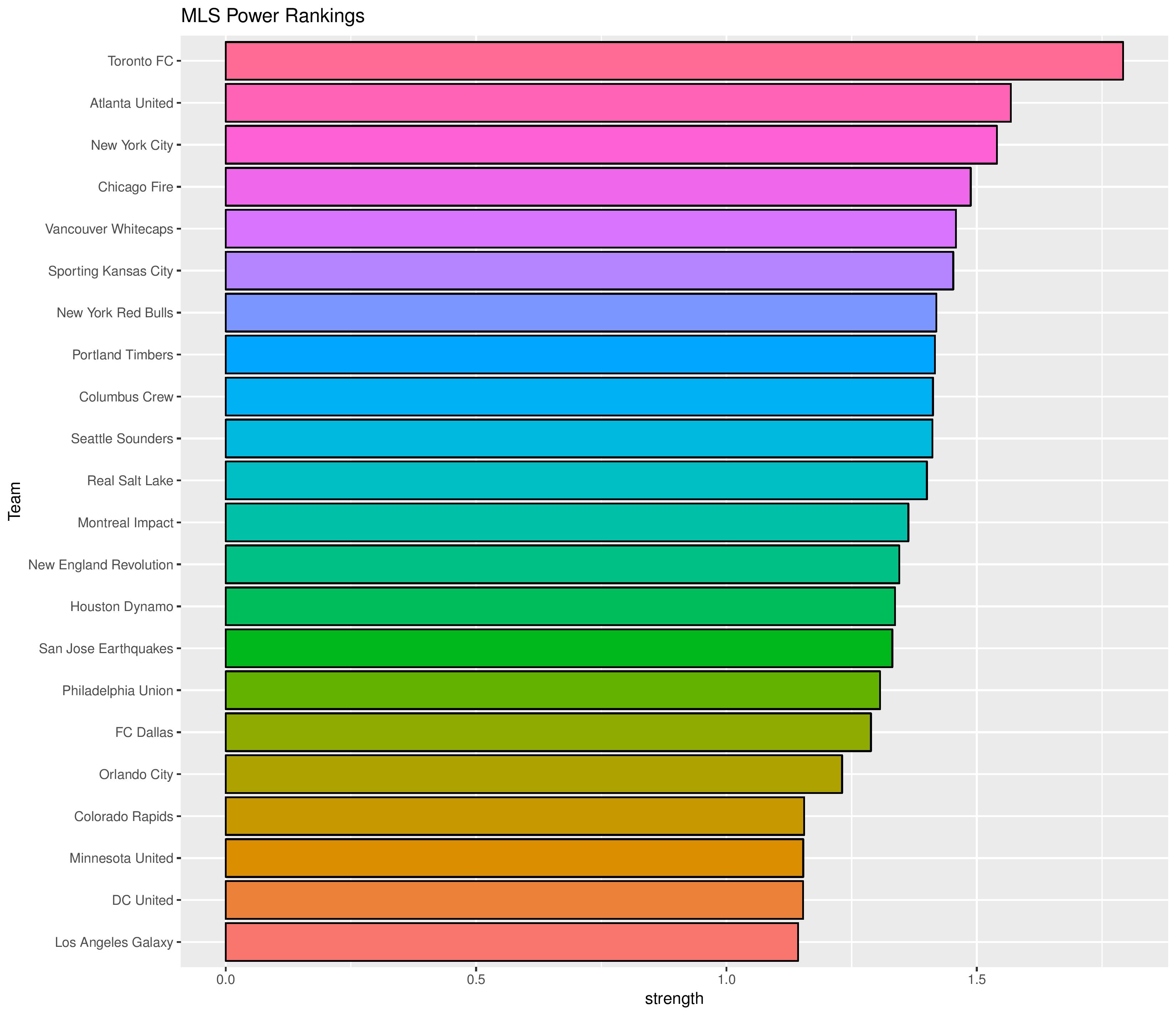
The “Power Rankings” we concoct are the “strength” of the team according to its competitive expectations. They are computed by forecasting the expected points (3 x win probability + 1 x draw probability) against every other MLS team – both home and away – and taking the average per team.
SEBA has the Union declining from 15th to 16th while ESPN has the Union climbing to 14th from 16th. Meanwhile, Soccer America has Philadelphia dropping from 19th to 20th, MLSSoccer has the Union jumping from 17th to 16th, and SI has Philadelphia moving up from 18th to 17th.
For those interested in how Philadelphia’s matches are weighted in the model (especially if skeptical about why SEBA’s rankings can be different from other outlets):
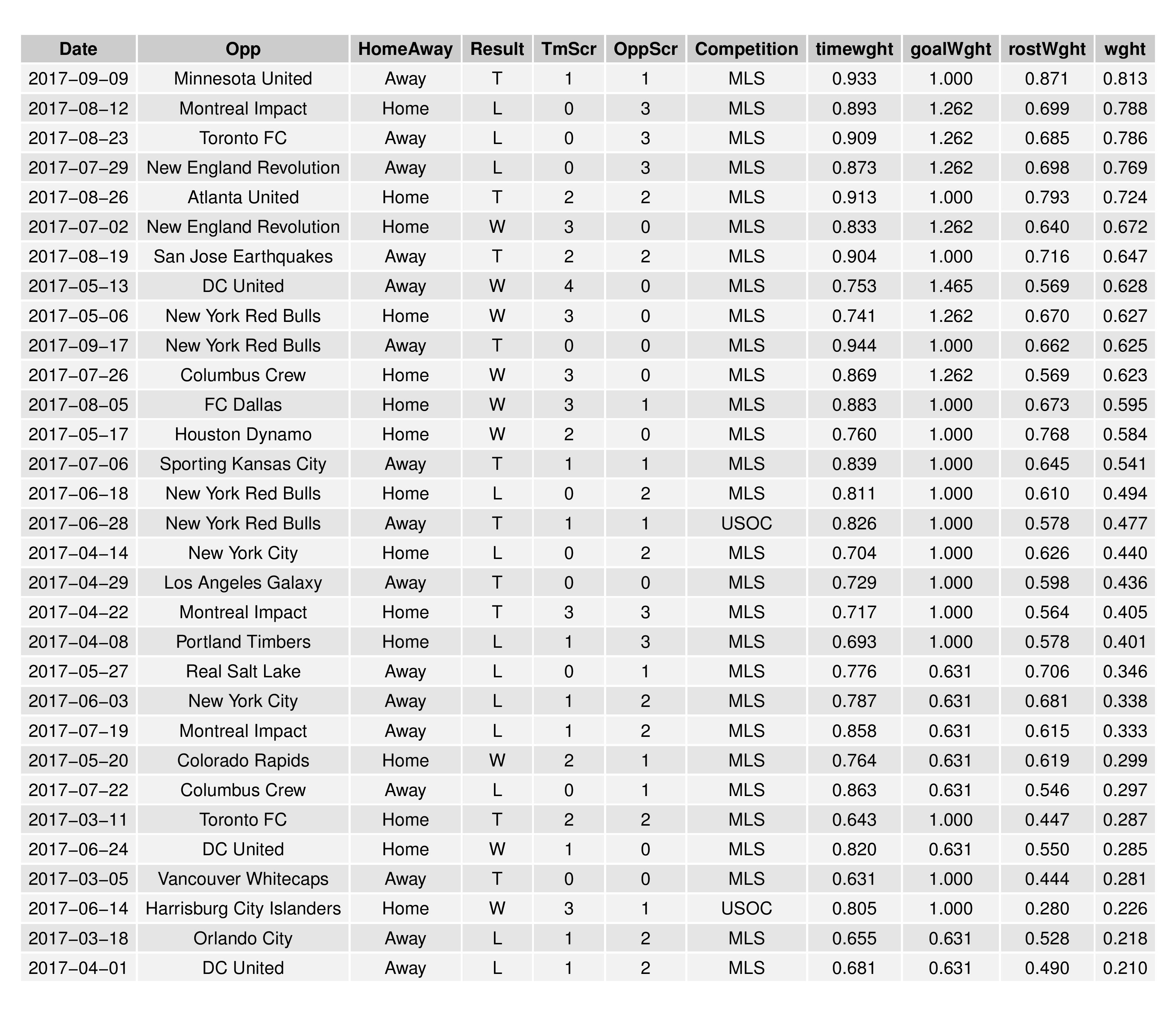
‘wght’ is the actual weight value used in the model, which is a combination of the ‘timewght’ (how long ago the match occurred), ‘goalWght’ (how much luck could have influenced the match result, as indicated by the goal differential), and ‘rostWght’ (how similar the roster deployments for both teams were compared with current trends).
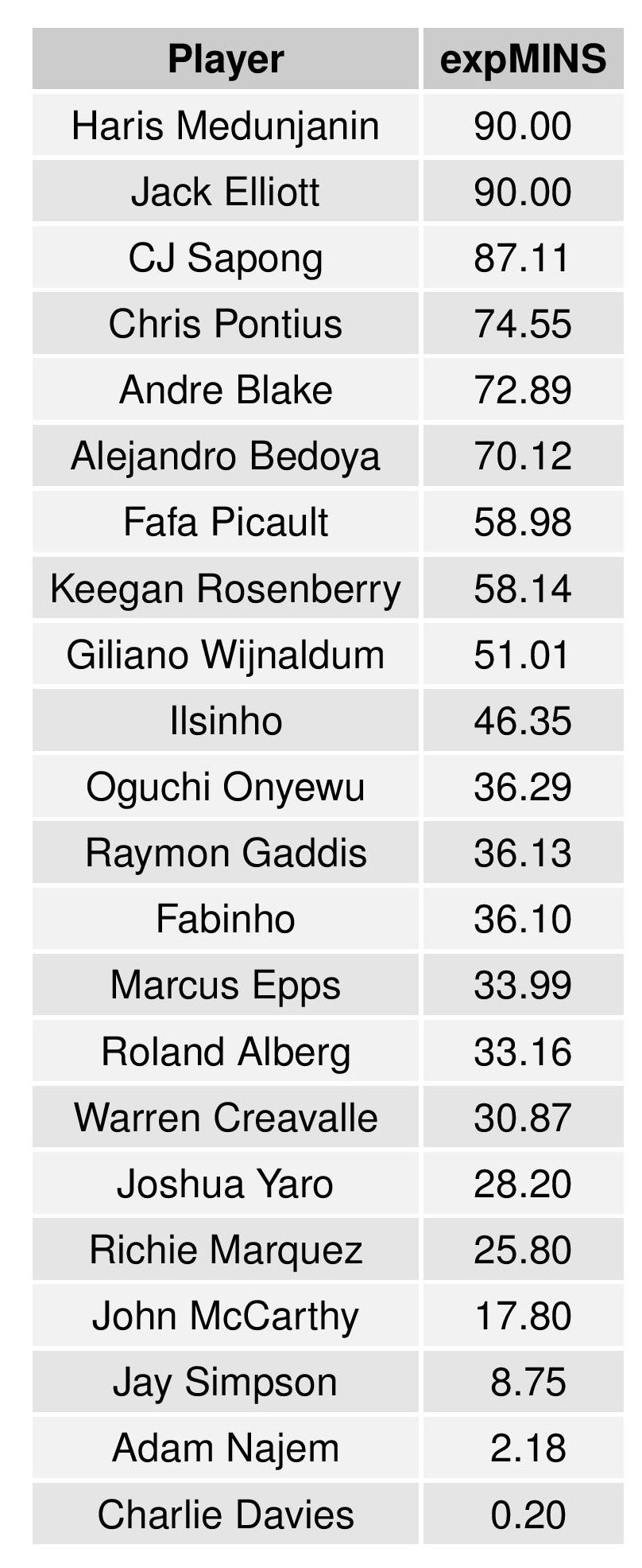
By comparison, the current roster expectations for maximum weight for the Union (and therefore the model’s assessment of ‘who’ Philadelphia is in the model) are currently:
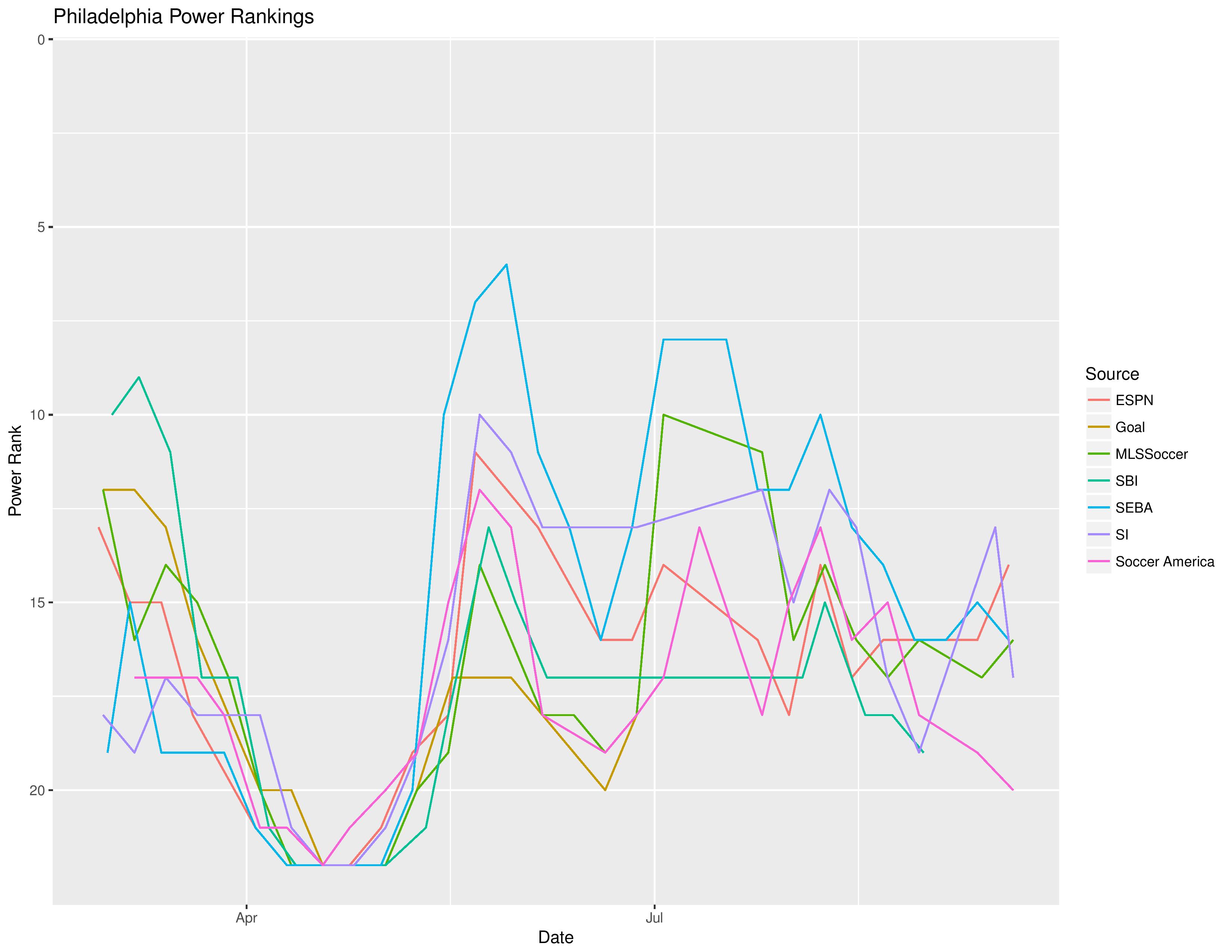
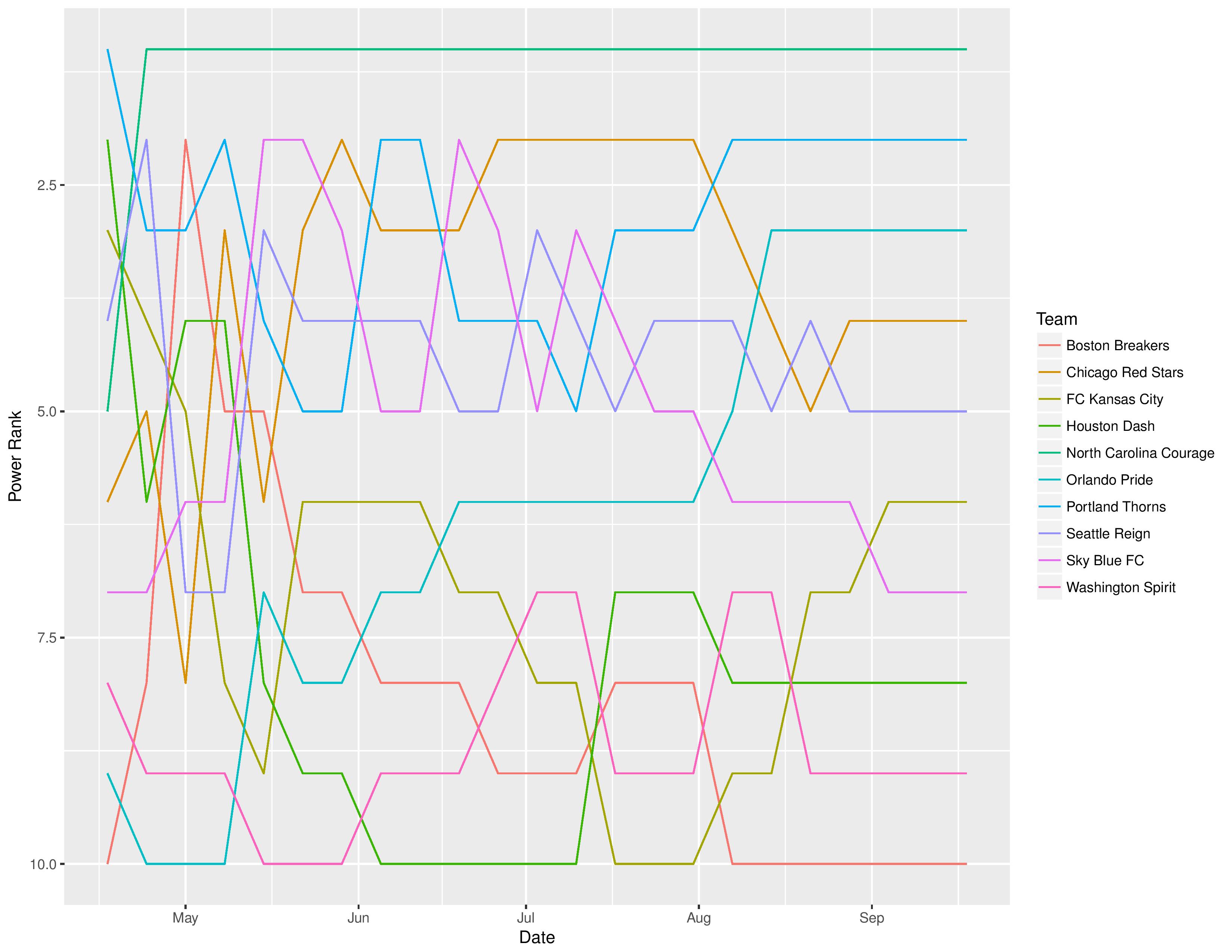
The following shows the evolution of SEBA’s power rankings for the MLS Eastern Conference over time:

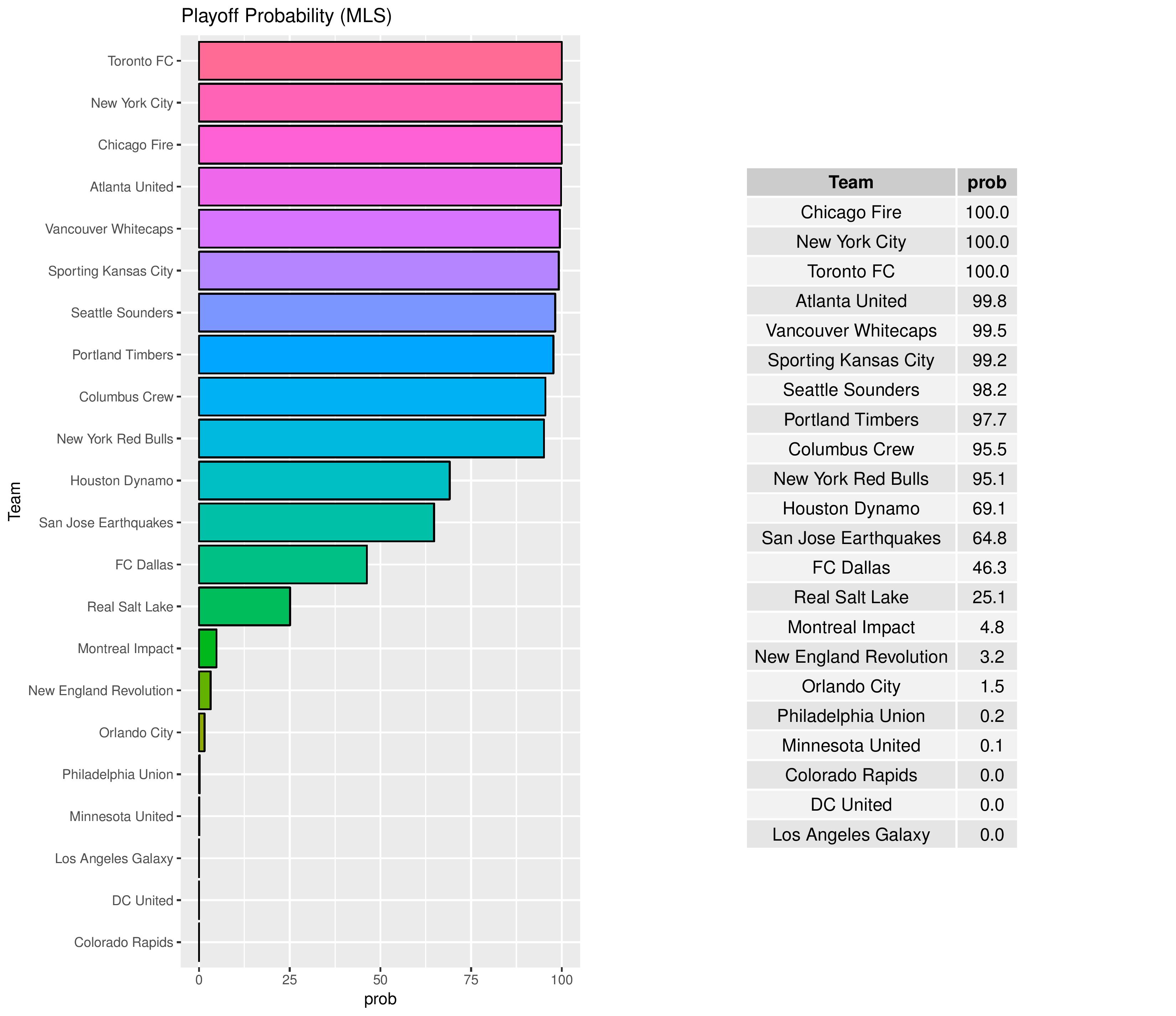
Playoffs probability and more
Philadelphia’s playoffs odds have decreased from 0.3% to 0.2%.
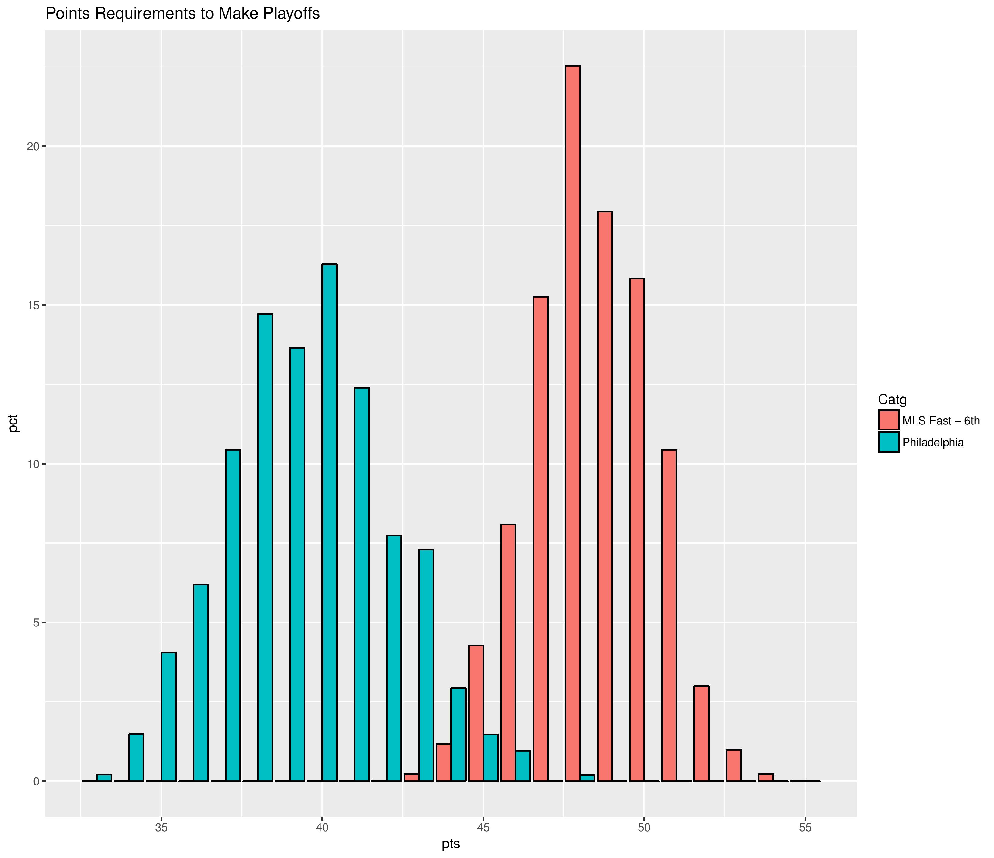
The following shows the simulation distribution for the points earned by the sixth place MLS East club as well as the simulation distribution of points that Philadelphia is expected to earn.
Tiebreakers aside, the Union make the playoffs when >= this MLS Eastern Conference 6th place value.
The most common number of points required to make the playoffs in the East’s 6th slot declined from 49 to 48 while the most common number of points simulated for the Union has increased from 39 to 40.
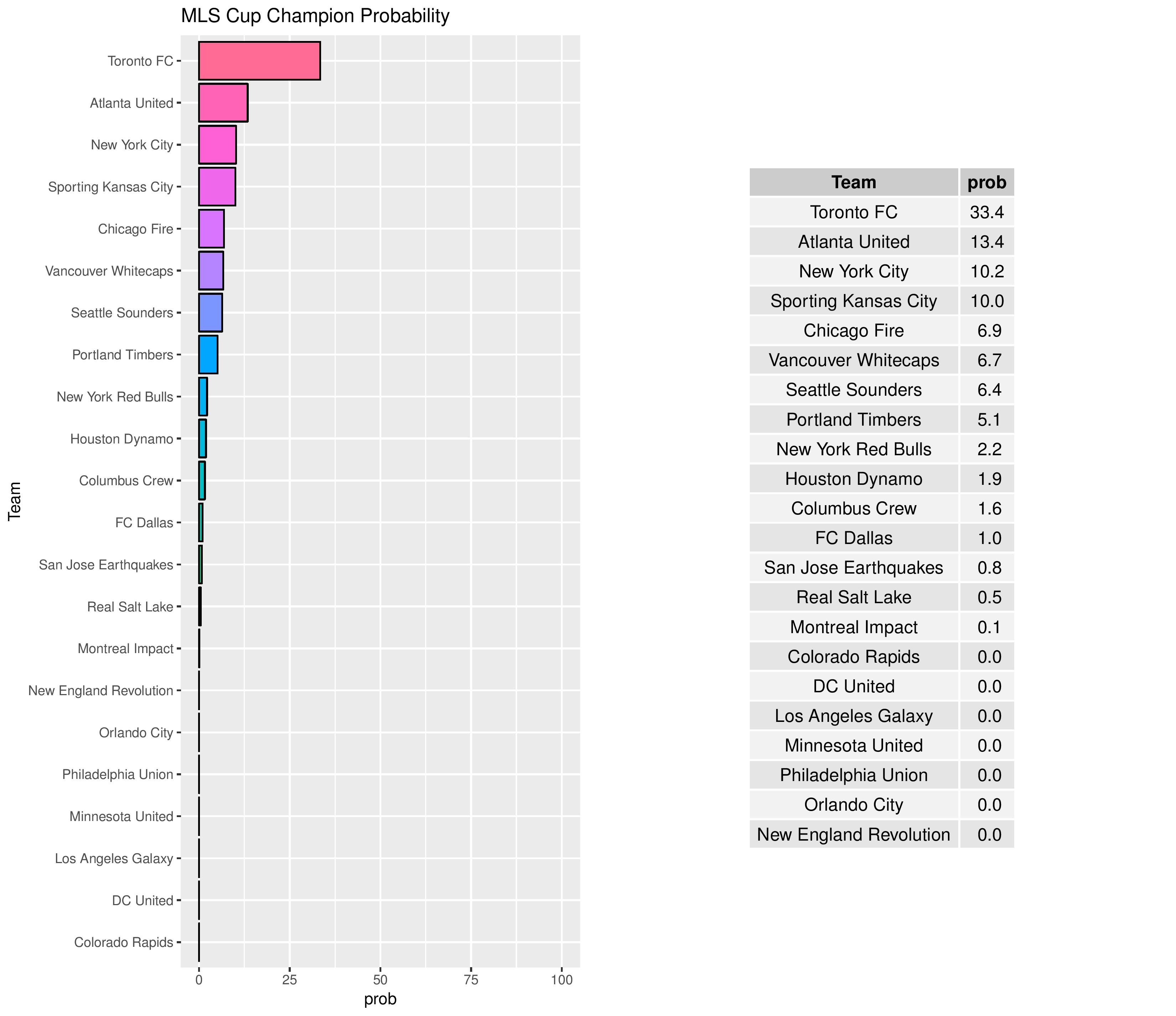
In part, clubs that score a lot of goals are given an advantage in MLS Cup due to the two-leg aggregate goal format of the conference semifinals and finals. That gives those clubs a better chance at notching large victories which carry over.
The Union’s chances of winning the MLS Cup remain at practically zero.
In the U.S. Open Cup, poor teams with a higher propensity to earn a draw are given an advantage as they are more likely to reach penalty kicks, which are a complete tossup. Conversely, good teams with a higher propensity to earn a draw have a disadvantage for the same reason.

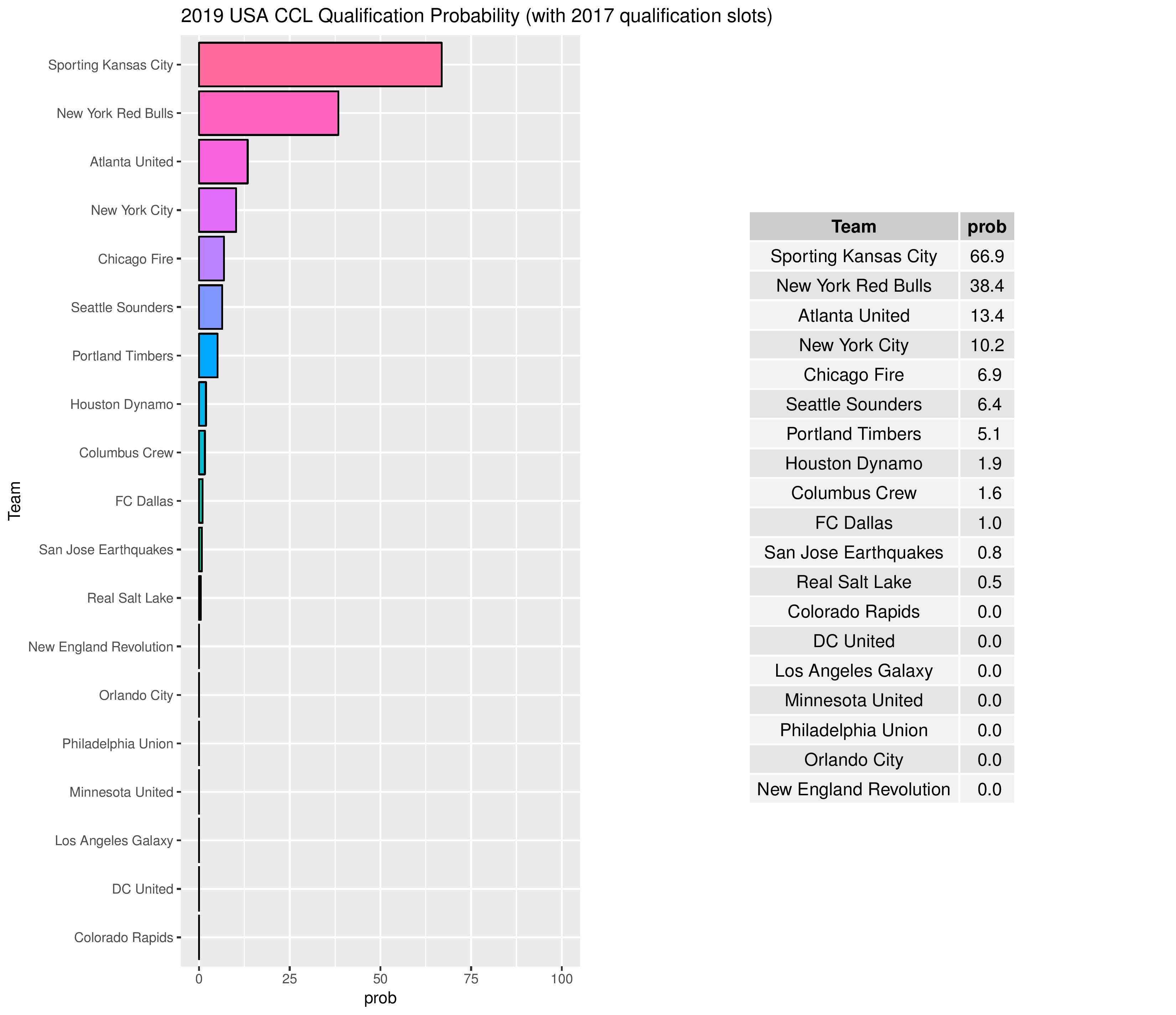
Philadelphia’s chances for qualifying in 2017 for the 2019 edition of the CONCACAF Champions League remain at practically zero.
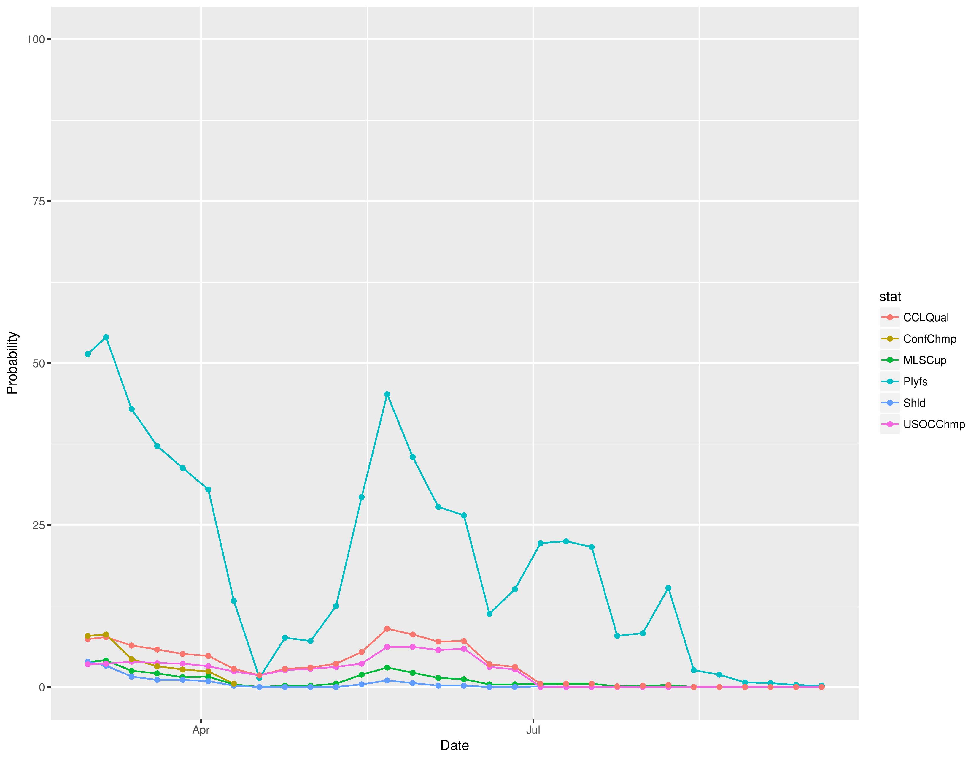
Over time, we can see how Philadelphia’s odds for different prizes have changed:
The following are probabilities for each category of outcomes for Philadelphia:
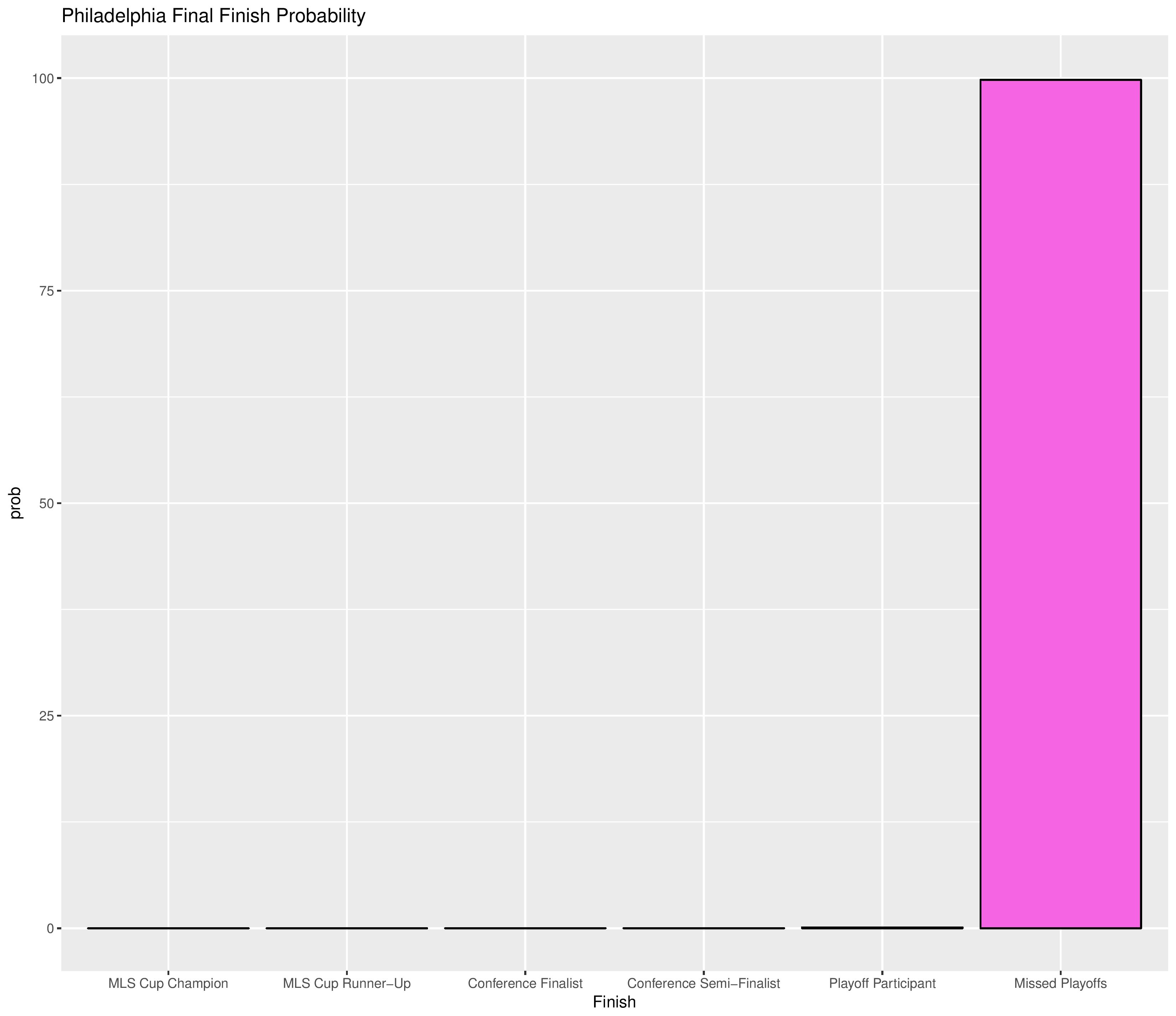
The following shows the probability of each playoff ranking finish:

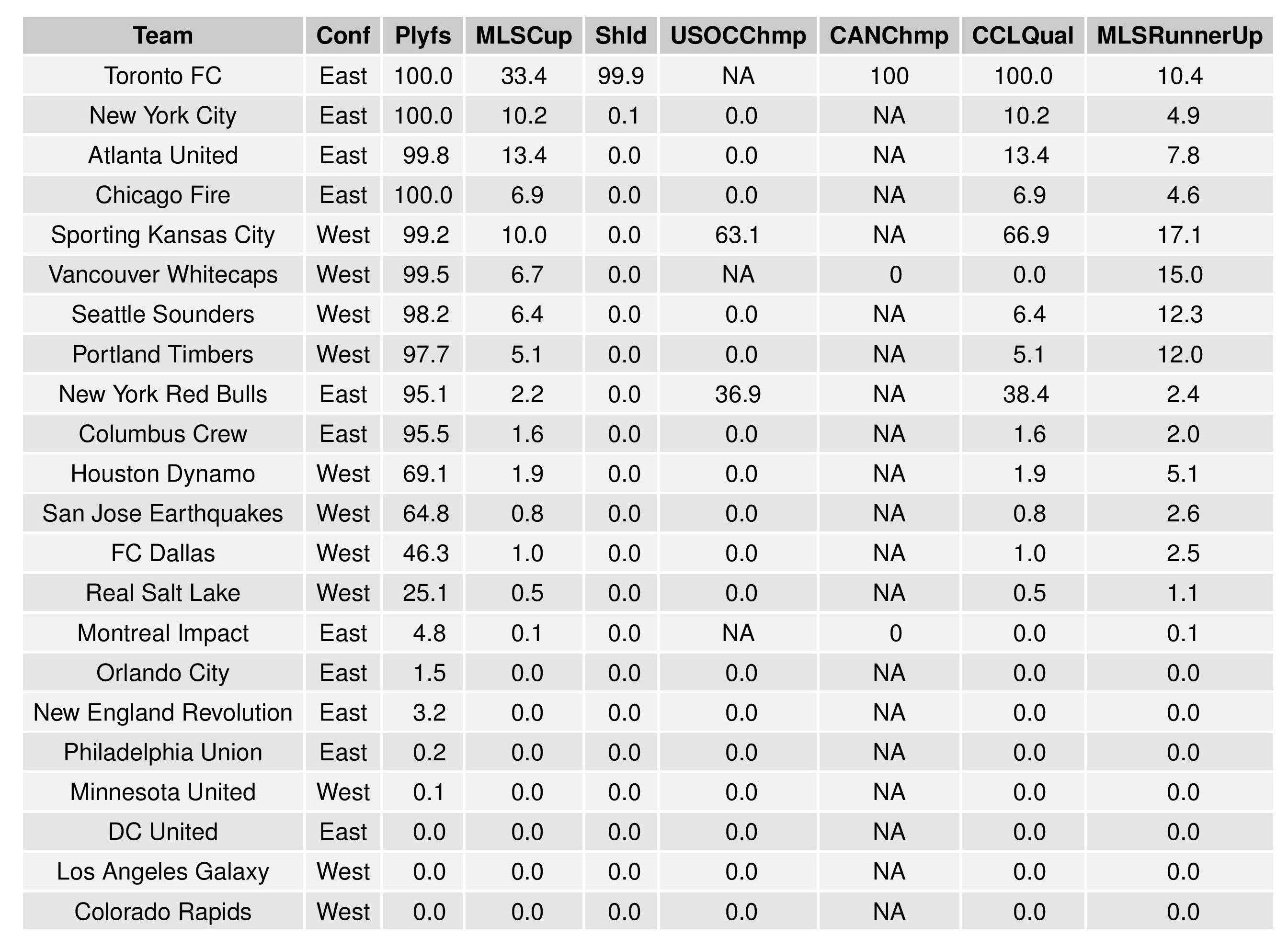
The following shows the summary of the simulations in an easy table format:

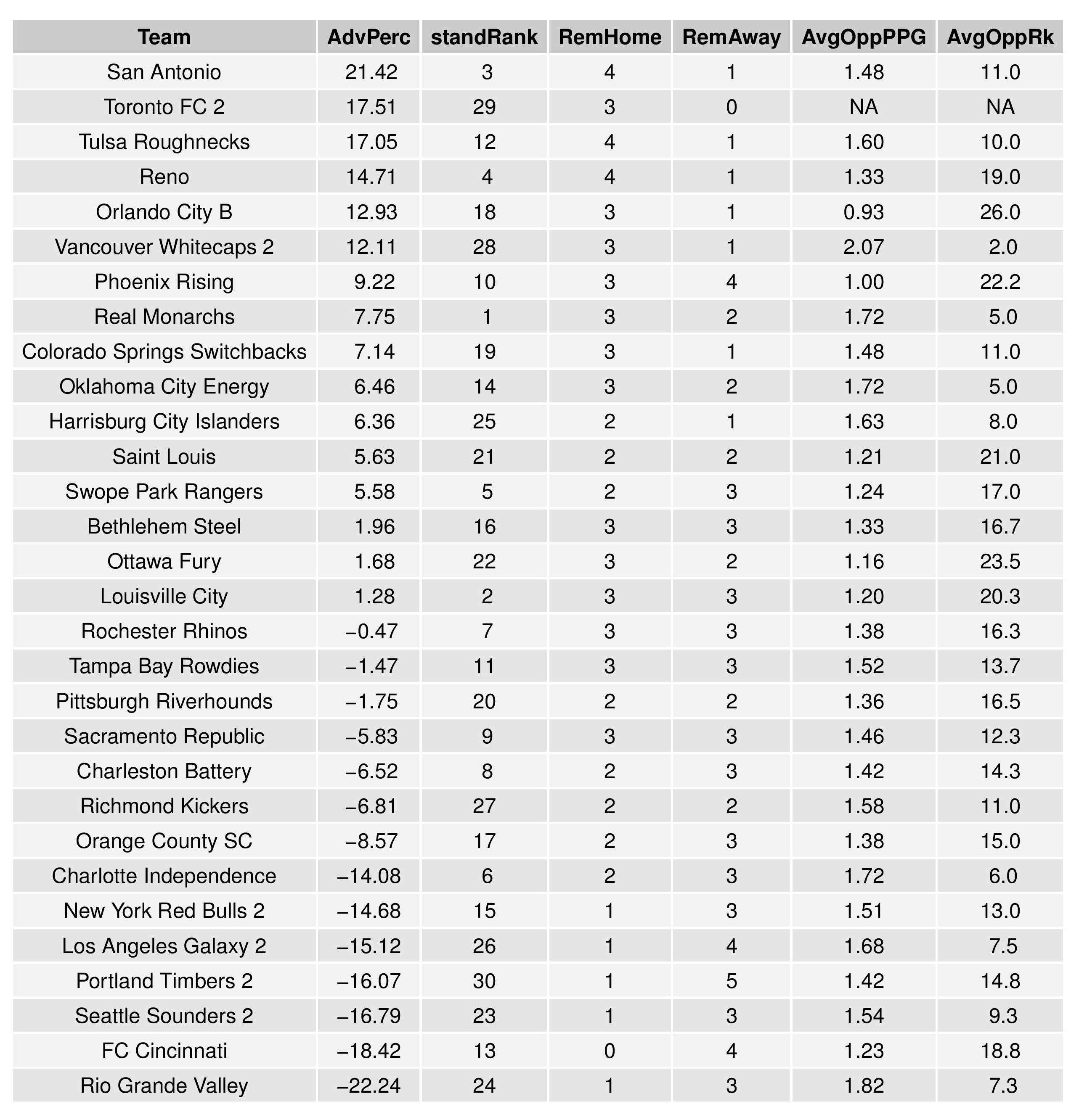
Next, we show how the Remaining Strength of Schedule affects each team.
The “Points Percentage Advantage” shown on the X-axis represents the percentage of points expected over the league average schedule. This “points expected” value is generated by simulating how all teams would perform with all remaining schedules (and therefore judges a schedule based upon how all teams would perform in that scenario).
In short, the higher the value, the easier the remaining schedule.
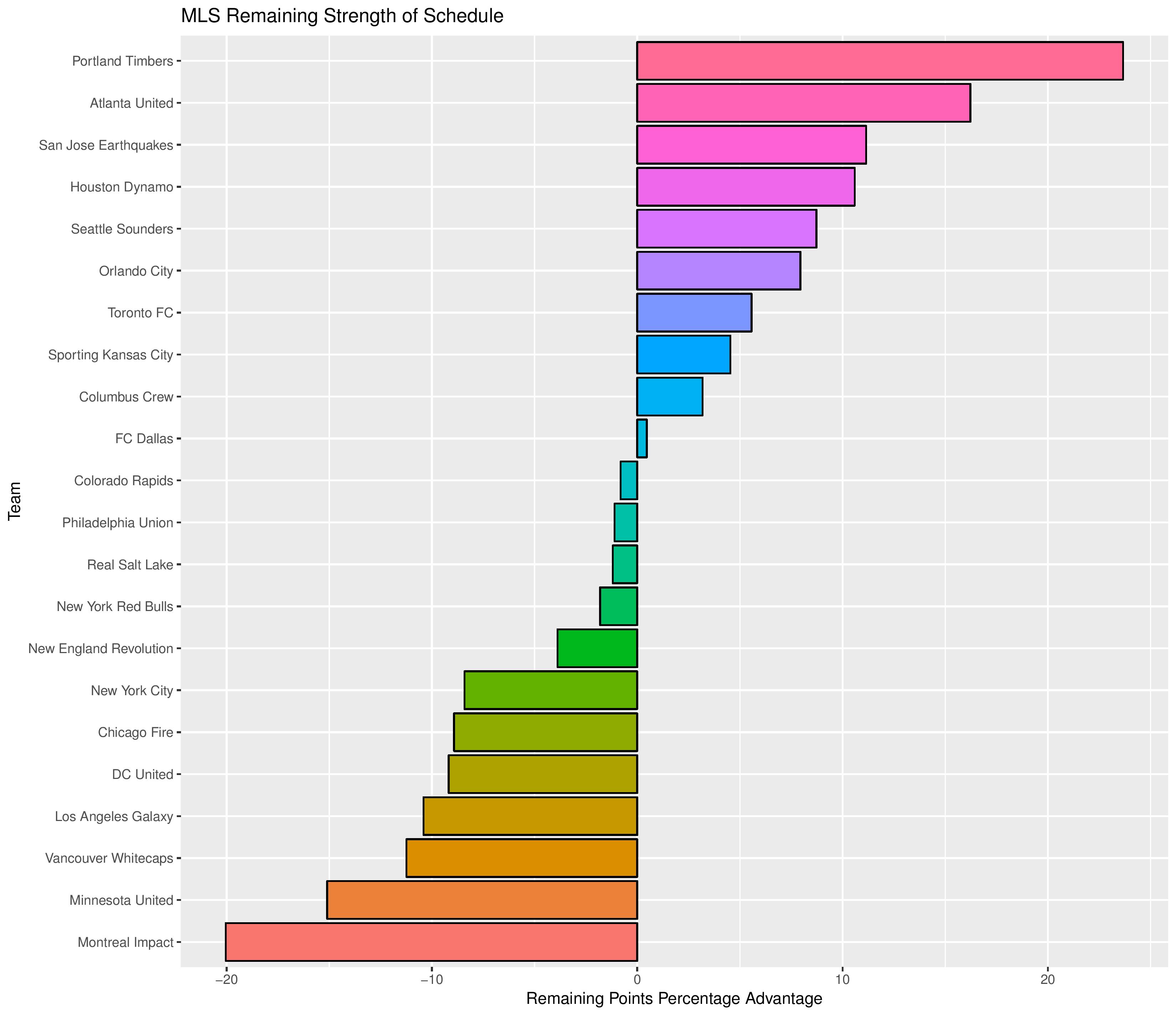
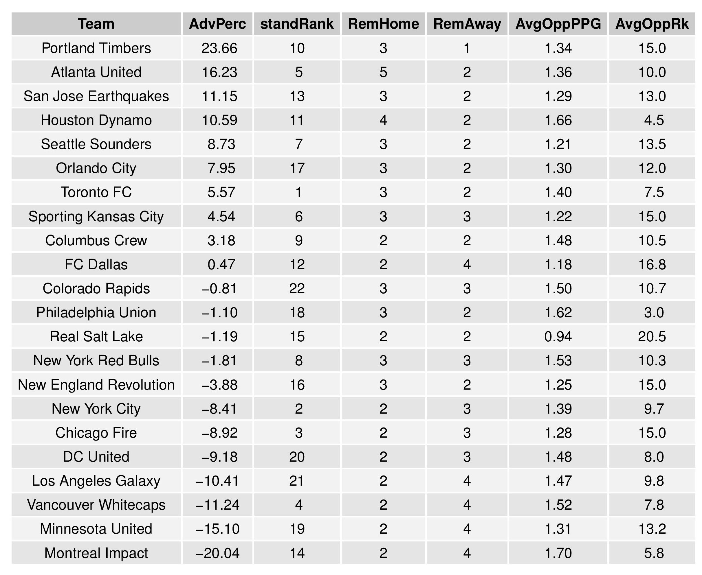
Accompanying the advantage percentage in the following table is their current standings rank (right now ties are not properly calculated beyond pts/gd/gf; I may fix that, but maybe not for a while), the remaining home matches, the remaining away matches, the current average points-per-game of future opponents (results-based, not model-based), and the average power ranking of future opponents according to SEBA.
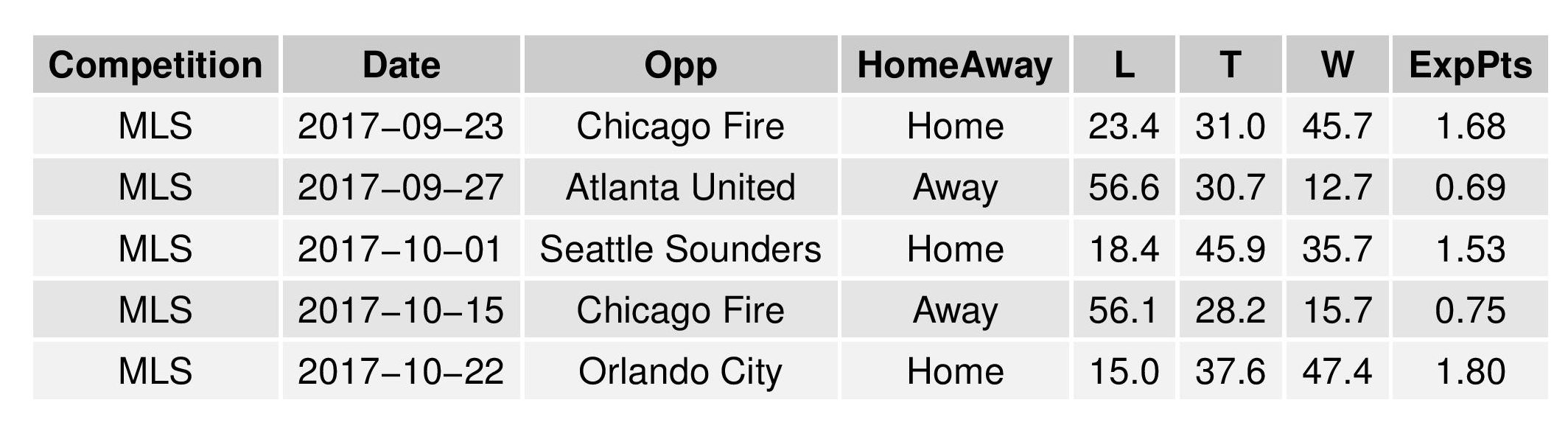
The following shows the expectations for upcoming Philadelphia matches:
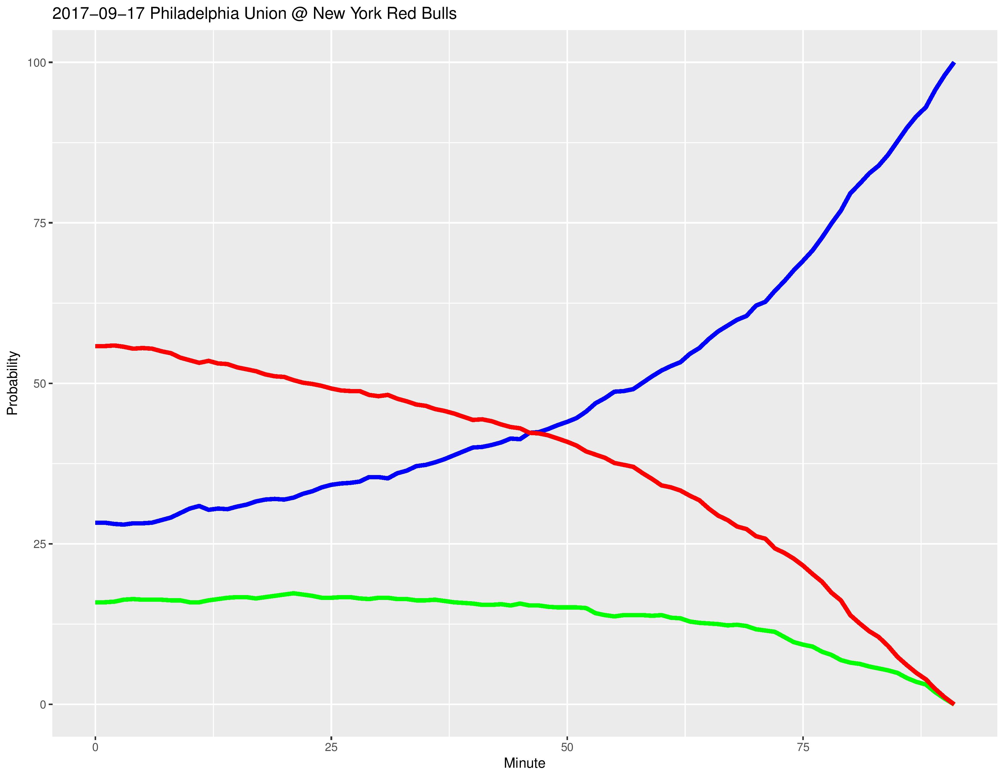
Last Game Probability Chart
This model finally incorporates changing team statistics due to subs and yellow/red cards.
For the following, the green line represents the odds of a win, the blue line the odds of a tie, and the red line the odds of a loss.
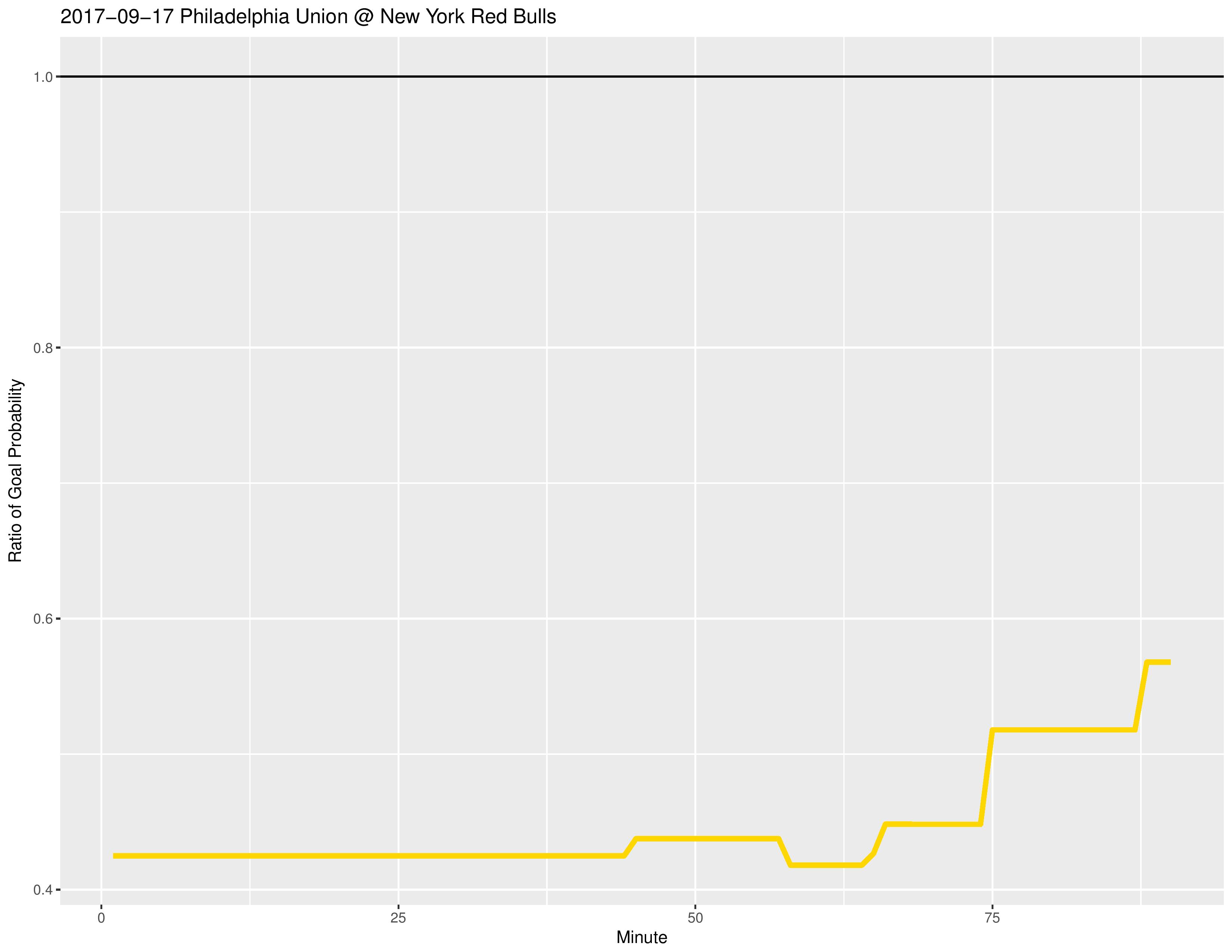
The following shows the changing proportion of Philadelphia’s probability of scoring goals compared with their opponents’. This proportion can only change due to subs, yellow cards, and red cards.
*For example, a value of 2 means that Philadelphia is twice as likely to score as its opponent. A value of 0.5 means that Philadelphia is half as likely to score as its opponent.
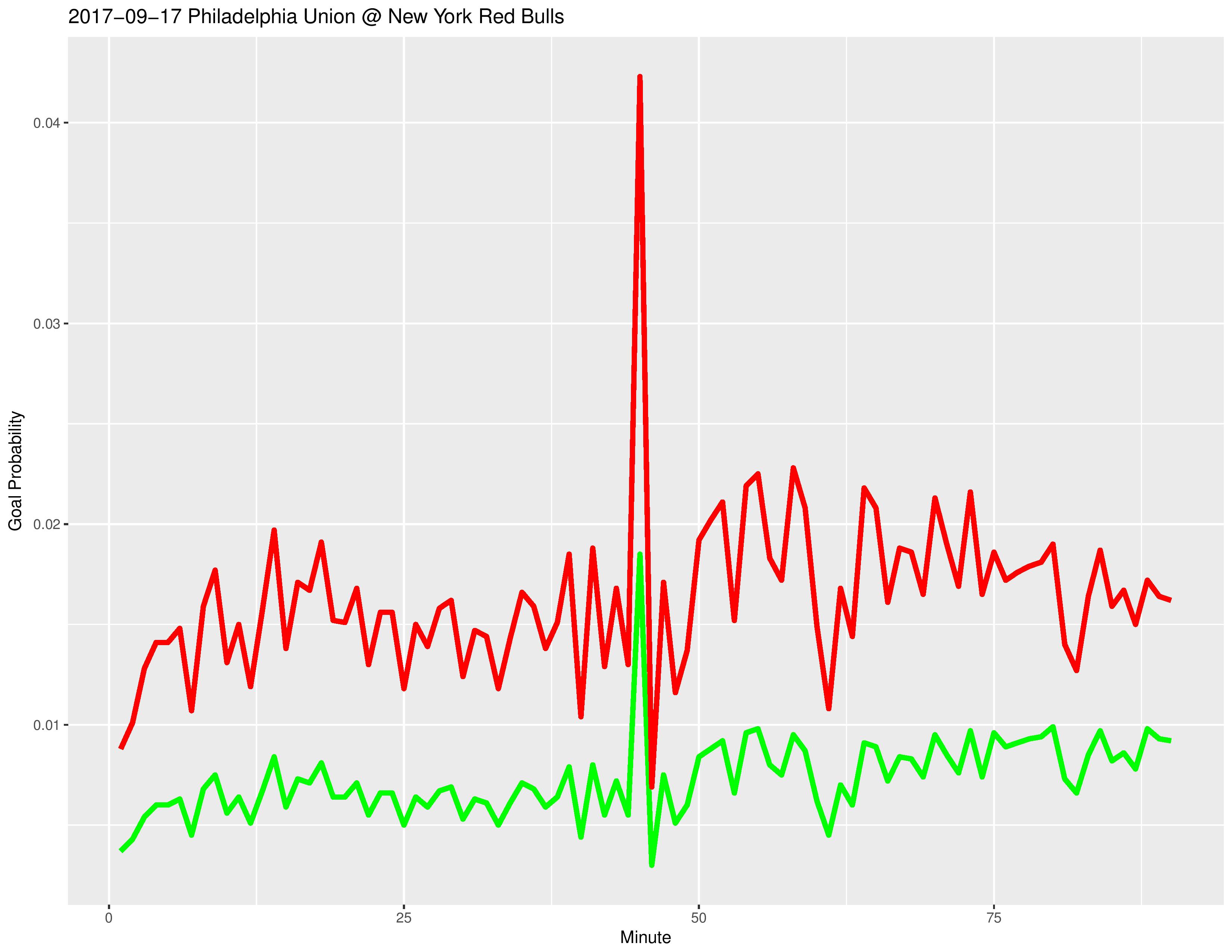
The following shows the changing raw probability of the two teams each scoring a goal. Green is Philadelphia’s probability of scoring a goal and red is their opponent’s probability of scoring a goal.
The reason for the spike at the 45th minute is because ’45+x’ is condensed to the 45th minute (therefore increasing the frequency of goals occurring in the 45th minute) to avoid duplication with the actual 46th/47th/etc minute, whereas the same situation does not occur for ’90+x’ minute, for which we actually calculate the addition and attribute the action to the goals to the 91st/92nd/etc minute if they occur.
Philadelphia +/- Player Analysis
The ‘+’ is a measure counting how many goals were scored by the Union while the player was on the field. The ‘-‘ counts how many goals were scored against the Union while the player was on the field.
The first table is for 2017. The second table is for all-time since 2013.
| Player | Net | + | – | MINS | Net/90 | +/90 | -/90 | |
|---|---|---|---|---|---|---|---|---|
| 1 | Chris Pontius | 7 | 29 | 22 | 4064 | 0.155 | 0.642 | 0.487 |
| 2 | Oguchi Onyewu | 5 | 29 | 24 | 4770 | 0.094 | 0.547 | 0.453 |
| 3 | Jack Elliott | 4 | 32 | 28 | 5294 | 0.068 | 0.544 | 0.476 |
| 4 | Giliano Wijnaldum | 3 | 19 | 16 | 3087 | 0.087 | 0.554 | 0.466 |
| 5 | Warren Creavalle | 2 | 5 | 3 | 514 | 0.350 | 0.875 | 0.525 |
| 6 | Derrick Jones | 1 | 10 | 9 | 1469 | 0.061 | 0.613 | 0.551 |
| 7 | Raymon Gaddis | 1 | 26 | 25 | 4530 | 0.020 | 0.517 | 0.497 |
| 8 | Andre Blake | 1 | 27 | 26 | 4770 | 0.019 | 0.509 | 0.491 |
| 9 | CJ Sapong | 0 | 36 | 36 | 6280 | 0.000 | 0.516 | 0.516 |
| 10 | Ilsinho | 0 | 22 | 22 | 3160 | 0.000 | 0.627 | 0.627 |
| 11 | Fabian Herbers | 0 | 8 | 8 | 660 | 0.000 | 1.091 | 1.091 |
| 12 | Alejandro Bedoya | -1 | 30 | 31 | 5457 | -0.016 | 0.495 | 0.511 |
| 13 | Roland Alberg | -1 | 14 | 15 | 1668 | -0.054 | 0.755 | 0.809 |
| 14 | Haris Medunjanin | -2 | 37 | 39 | 6831 | -0.026 | 0.487 | 0.514 |
| 15 | Adam Najem | -2 | 1 | 3 | 142 | -1.268 | 0.634 | 1.901 |
| 16 | John McCarthy | -3 | 10 | 13 | 2070 | -0.130 | 0.435 | 0.565 |
| 17 | Fabinho | -4 | 18 | 22 | 3600 | -0.100 | 0.450 | 0.550 |
| 18 | Fafa Picault | -4 | 21 | 25 | 3517 | -0.102 | 0.537 | 0.640 |
| 19 | Keegan Rosenberry | -4 | 11 | 15 | 2077 | -0.173 | 0.477 | 0.650 |
| 20 | Joshua Yaro | -4 | 5 | 9 | 942 | -0.382 | 0.478 | 0.860 |
| 21 | Marcus Epps | -5 | 5 | 10 | 824 | -0.546 | 0.546 | 1.092 |
| 22 | Jay Simpson | -5 | 4 | 9 | 350 | -1.286 | 1.029 | 2.314 |
| 23 | Richie Marquez | -8 | 8 | 16 | 1953 | -0.369 | 0.369 | 0.737 |
| Player | Net | + | – | MINS | Net/90 | +/90 | -/90 | |
|---|---|---|---|---|---|---|---|---|
| 1 | Antoine Hoppenot | 7 | 21 | 14 | 1008 | 0.625 | 1.875 | 1.250 |
| 2 | Conor Casey | 7 | 64 | 57 | 8348 | 0.075 | 0.690 | 0.615 |
| 3 | Oguchi Onyewu | 5 | 29 | 24 | 4770 | 0.094 | 0.547 | 0.453 |
| 4 | Jack McInerney | 5 | 35 | 30 | 5403 | 0.083 | 0.583 | 0.500 |
| 5 | Chris Pontius | 5 | 73 | 68 | 11411 | 0.039 | 0.576 | 0.536 |
| 6 | Jack Elliott | 4 | 32 | 28 | 5294 | 0.068 | 0.544 | 0.476 |
| 7 | Fred | 3 | 8 | 5 | 689 | 0.392 | 1.045 | 0.653 |
| 8 | Giliano Wijnaldum | 3 | 19 | 16 | 3087 | 0.087 | 0.554 | 0.466 |
| 9 | Brian Brown | 2 | 6 | 4 | 328 | 0.549 | 1.646 | 1.098 |
| 10 | Ethan White | 2 | 36 | 34 | 6056 | 0.030 | 0.535 | 0.505 |
| 11 | Matt Kassel | 1 | 2 | 1 | 139 | 0.647 | 1.295 | 0.647 |
| 12 | Matthew Jones | 1 | 3 | 2 | 450 | 0.200 | 0.600 | 0.400 |
| 13 | Gabriel Farfan | 1 | 6 | 5 | 643 | 0.140 | 0.840 | 0.700 |
| 14 | Derrick Jones | 1 | 10 | 9 | 1469 | 0.061 | 0.613 | 0.551 |
| 15 | Ilsinho | 1 | 48 | 47 | 6333 | 0.014 | 0.682 | 0.668 |
| 16 | Warren Creavalle | 0 | 37 | 37 | 5665 | 0.000 | 0.588 | 0.588 |
| 17 | Michael Lahoud | 0 | 36 | 36 | 5294 | 0.000 | 0.612 | 0.612 |
| 18 | Fabian Herbers | 0 | 34 | 34 | 3711 | 0.000 | 0.825 | 0.825 |
| 19 | Keon Daniel | 0 | 22 | 22 | 3481 | 0.000 | 0.569 | 0.569 |
| 20 | Carlos Valdés | 0 | 11 | 11 | 1946 | 0.000 | 0.509 | 0.509 |
| 21 | Bakary Soumaré | 0 | 3 | 3 | 504 | 0.000 | 0.536 | 0.536 |
| 22 | Zac MacMath | -1 | 88 | 89 | 15930 | -0.006 | 0.497 | 0.503 |
| 23 | Vincent Nogueira | -1 | 81 | 82 | 13892 | -0.006 | 0.525 | 0.531 |
| 24 | Brian Sylvestre | -1 | 18 | 19 | 3330 | -0.027 | 0.486 | 0.514 |
| 25 | Austin Berry | -1 | 9 | 10 | 1667 | -0.054 | 0.486 | 0.540 |
| 26 | Rais Mbolhi | -1 | 1 | 2 | 270 | -0.333 | 0.333 | 0.667 |
| 27 | Walter Restrepo | -1 | 3 | 4 | 162 | -0.556 | 1.667 | 2.222 |
| 28 | Roger Torres | -1 | 1 | 2 | 68 | -1.324 | 1.324 | 2.647 |
| 29 | Corben Bone | -1 | 0 | 1 | 12 | -7.500 | 0.000 | 7.500 |
| 30 | Haris Medunjanin | -2 | 37 | 39 | 6831 | -0.026 | 0.487 | 0.514 |
| 31 | Jeff Parke | -2 | 37 | 39 | 6795 | -0.026 | 0.490 | 0.517 |
| 32 | Rais M’bolhi | -2 | 9 | 11 | 1800 | -0.100 | 0.450 | 0.550 |
| 33 | Pedro Ribeiro | -2 | 4 | 6 | 611 | -0.295 | 0.589 | 0.884 |
| 34 | Anderson Conceicão | -2 | 0 | 2 | 180 | -1.000 | 0.000 | 1.000 |
| 35 | Adam Najem | -2 | 1 | 3 | 142 | -1.268 | 0.634 | 1.901 |
| 36 | Charlie Davies | -2 | 2 | 4 | 52 | -3.462 | 3.462 | 6.923 |
| 37 | Raymond Lee | -2 | 0 | 2 | 24 | -7.500 | 0.000 | 7.500 |
| 38 | Sheanon Williams | -3 | 95 | 98 | 17177 | -0.016 | 0.498 | 0.513 |
| 39 | Leonardo Fernandes | -3 | 4 | 7 | 690 | -0.391 | 0.522 | 0.913 |
| 40 | Cristián Maidana | -4 | 62 | 66 | 10287 | -0.035 | 0.542 | 0.577 |
| 41 | Ken Tribbett | -4 | 33 | 37 | 5681 | -0.063 | 0.523 | 0.586 |
| 42 | Michael Farfan | -4 | 29 | 33 | 4822 | -0.075 | 0.541 | 0.616 |
| 43 | Joshua Yaro | -4 | 25 | 29 | 4288 | -0.084 | 0.525 | 0.609 |
| 44 | Fafa Picault | -4 | 21 | 25 | 3517 | -0.102 | 0.537 | 0.640 |
| 45 | Sébastien Le Toux | -5 | 119 | 124 | 19366 | -0.023 | 0.553 | 0.576 |
| 46 | Amobi Okugo | -5 | 87 | 92 | 16050 | -0.028 | 0.488 | 0.516 |
| 47 | Alejandro Bedoya | -5 | 43 | 48 | 7989 | -0.056 | 0.484 | 0.541 |
| 48 | Kléberson | -5 | 6 | 11 | 1303 | -0.345 | 0.414 | 0.760 |
| 49 | Marcus Epps | -5 | 5 | 10 | 824 | -0.546 | 0.546 | 1.092 |
| 50 | Jay Simpson | -5 | 4 | 9 | 350 | -1.286 | 1.029 | 2.314 |
| 51 | Tranquillo Barnetta | -6 | 54 | 60 | 9529 | -0.057 | 0.510 | 0.567 |
| 52 | Eric Ayuk | -6 | 19 | 25 | 3165 | -0.171 | 0.540 | 0.711 |
| 53 | Aaron Wheeler | -6 | 9 | 15 | 1730 | -0.312 | 0.468 | 0.780 |
| 54 | CJ Sapong | -7 | 105 | 112 | 18174 | -0.035 | 0.520 | 0.555 |
| 55 | Roland Alberg | -7 | 36 | 43 | 4468 | -0.141 | 0.725 | 0.866 |
| 56 | Zach Pfeffer | -7 | 15 | 22 | 2210 | -0.285 | 0.611 | 0.896 |
| 57 | Andre Blake | -8 | 82 | 90 | 15480 | -0.047 | 0.477 | 0.523 |
| 58 | Keegan Rosenberry | -8 | 64 | 72 | 11959 | -0.060 | 0.482 | 0.542 |
| 59 | Maurice Edu | -9 | 71 | 80 | 13587 | -0.060 | 0.470 | 0.530 |
| 60 | John McCarthy | -10 | 24 | 34 | 5220 | -0.172 | 0.414 | 0.586 |
| 61 | Leo Fernandes | -10 | 12 | 22 | 2082 | -0.432 | 0.519 | 0.951 |
| 62 | Danny Cruz | -11 | 47 | 58 | 7279 | -0.136 | 0.581 | 0.717 |
| 63 | Fabinho | -12 | 133 | 145 | 24158 | -0.045 | 0.495 | 0.540 |
| 64 | Fernando Aristeguieta | -12 | 13 | 25 | 2909 | -0.371 | 0.402 | 0.773 |
| 65 | Steven Vitória | -13 | 19 | 32 | 4410 | -0.265 | 0.388 | 0.653 |
| 66 | Andrew Wenger | -14 | 53 | 67 | 8723 | -0.144 | 0.547 | 0.691 |
| 67 | Richie Marquez | -15 | 87 | 102 | 16736 | -0.081 | 0.468 | 0.549 |
| 68 | Raymon Gaddis | -20 | 151 | 171 | 28749 | -0.063 | 0.473 | 0.535 |
| 69 | Brian Carroll | -21 | 119 | 140 | 22471 | -0.084 | 0.477 | 0.561 |
Model Validation
The following shows the overall net values since 2013 which is when data is available.
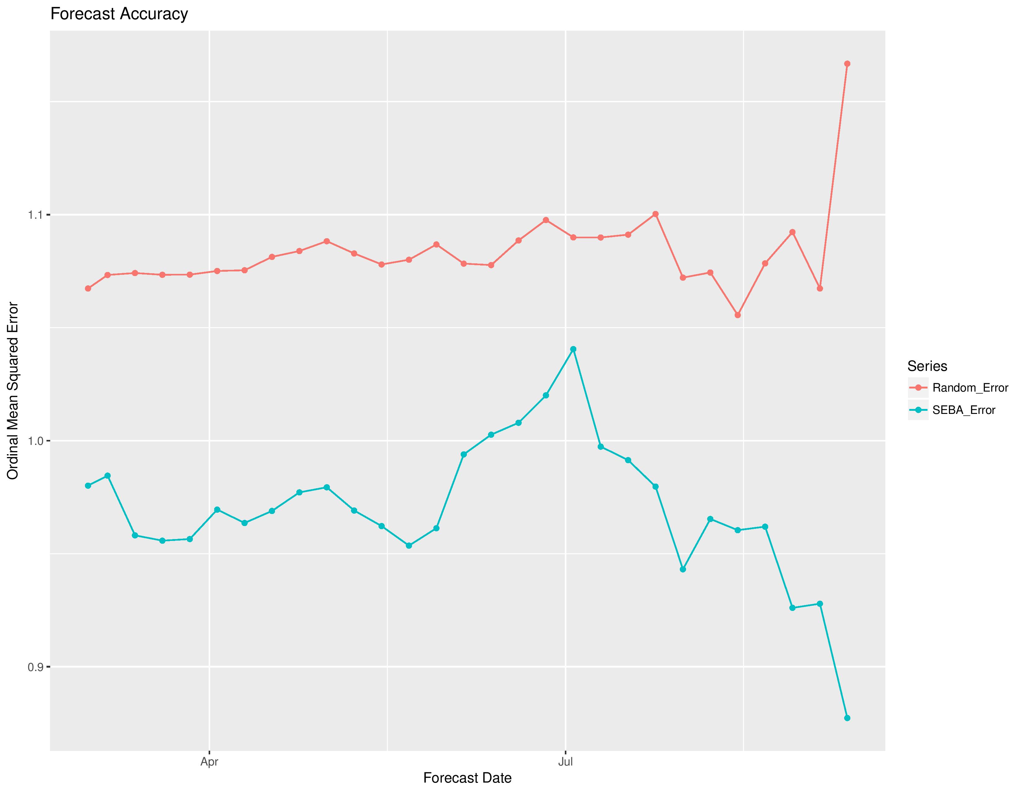
The following shows the degree of error by the model vs the error if the model was purely random without intelligence. The x-axis is based on the date from which the forecast was made (this will update throughout the season as more results are finalized and compared with predictions). The ordinal squared error metric (not a traditional metric) is calculated as:
(ProbW – ActW)^2 + (ProbT – ActT)^2 + (ProbL – ActL)^2 +
((ProbW + ProbT) – (ActW + ActT))^2 +
((ProbL + ProbT) – (ActL + ActT))^2
where Prob[W/T/L] is the model’s probability of resulting outcomes and Act[W/T/L] is a 1 or 0 representation of whether it actually happened.
Random errors will decline when more ties occur as there is a less severe penalty for ties.
We should expect random errors to remain relatively constant over time, where our model’s errors will hopefully decline as the season goes on as it gathers new information.
These data points are not fixed until the end of the season due to additional matches adding to them.
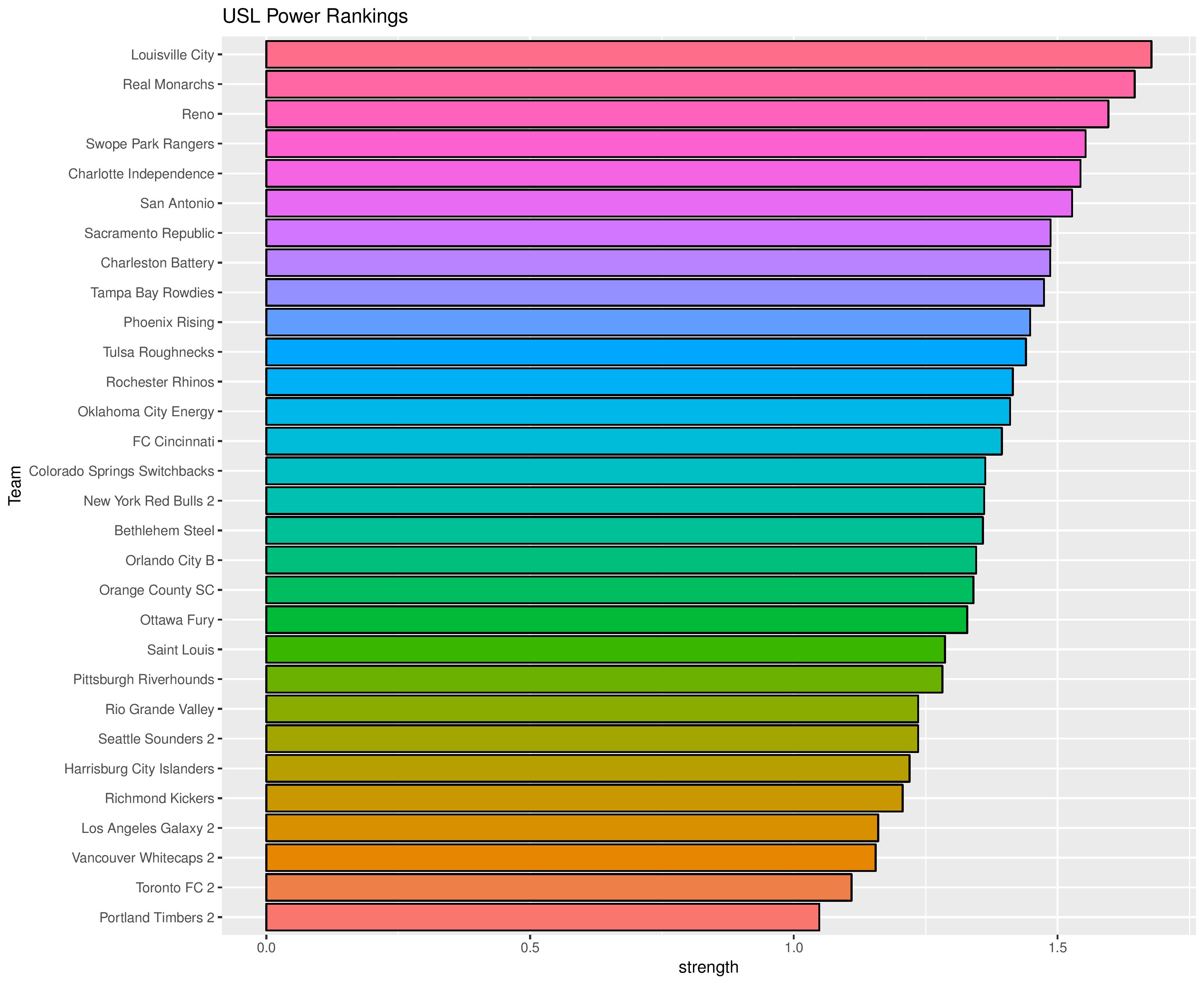
USL
Power Rankings
SEBA has the Bethlehem Steel climbing to 17th from 18th while it has Harrisburg City hopping back to 25th from 26th.
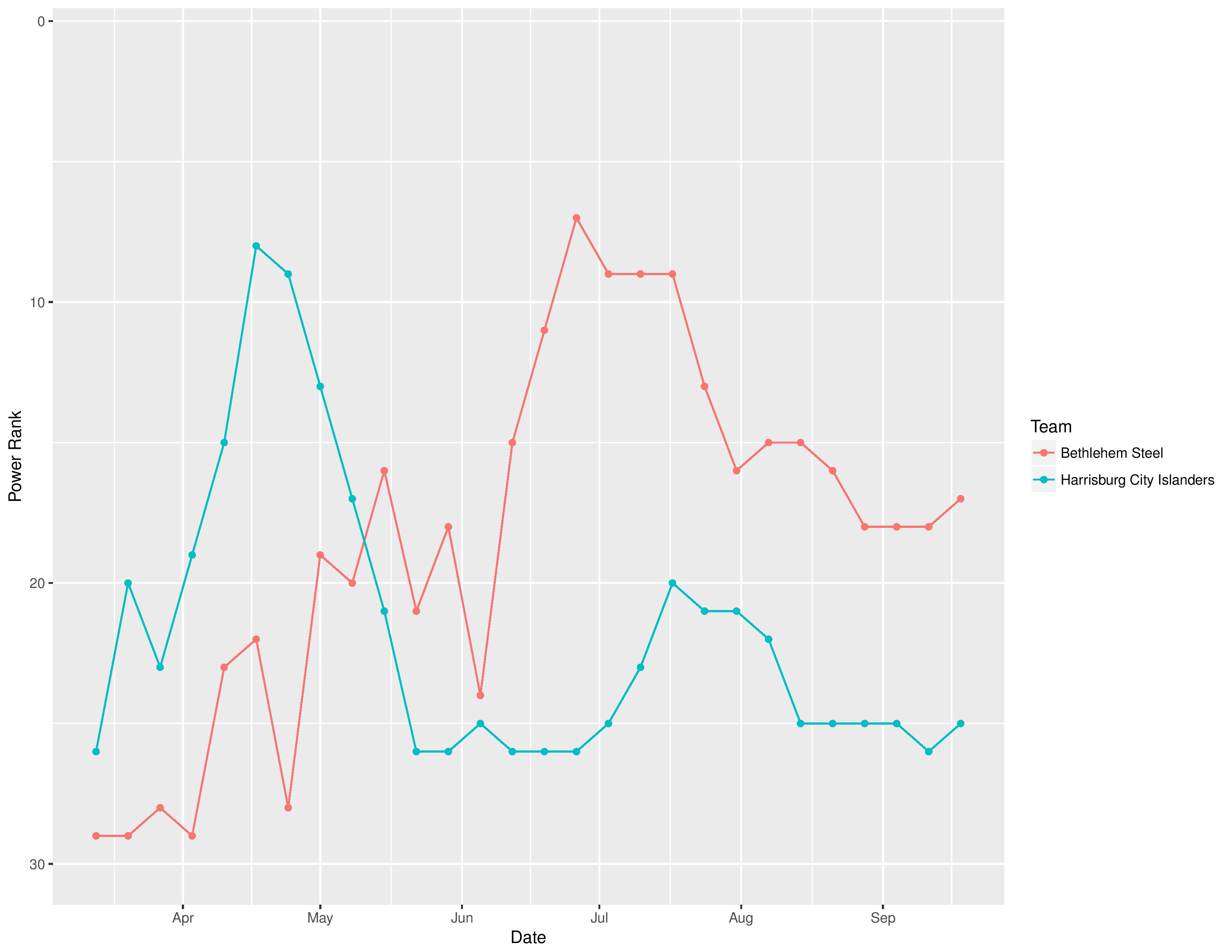
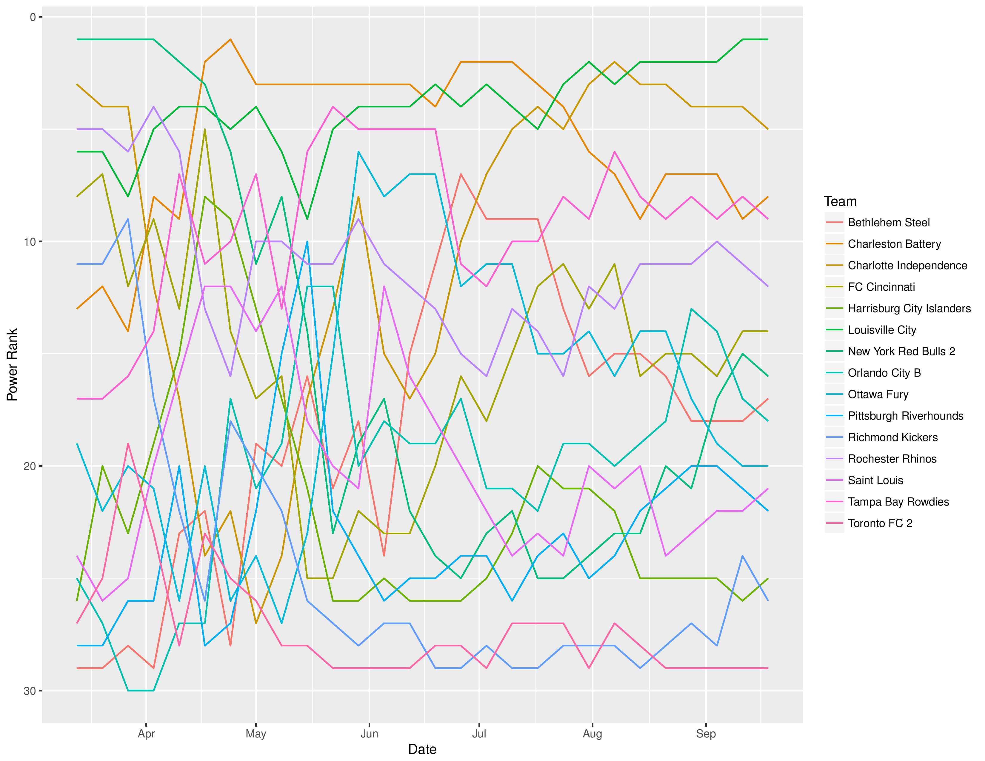
The following shows the evolution of SEBA’s power rankings for the USL East over time.
Playoffs probability and more
Bethlehem’s playoff odds have increased from 65.1% to 71.1% while Harrisburg City’s odds of reaching the postseason decreased from 0.4% to 0.1%.

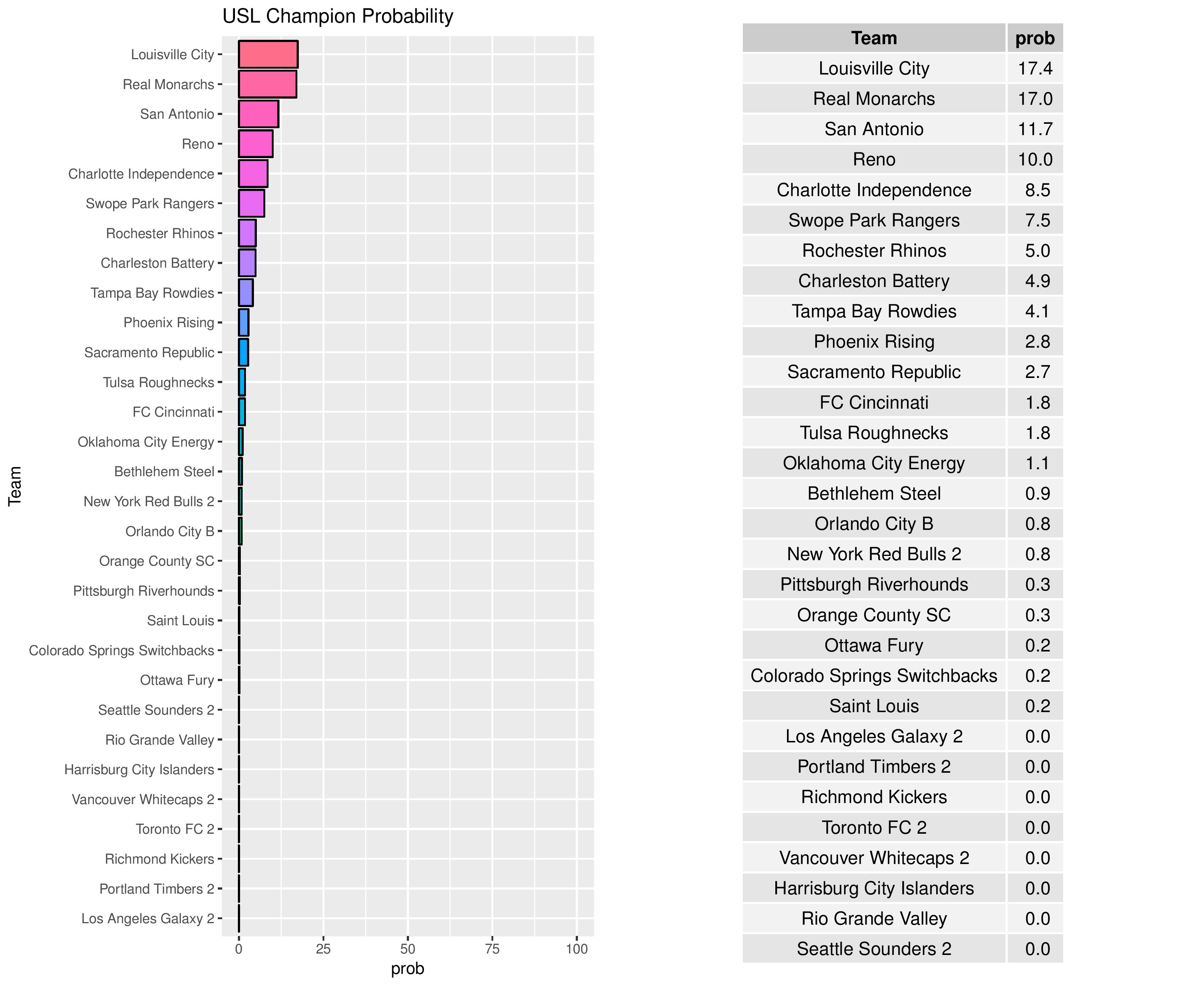
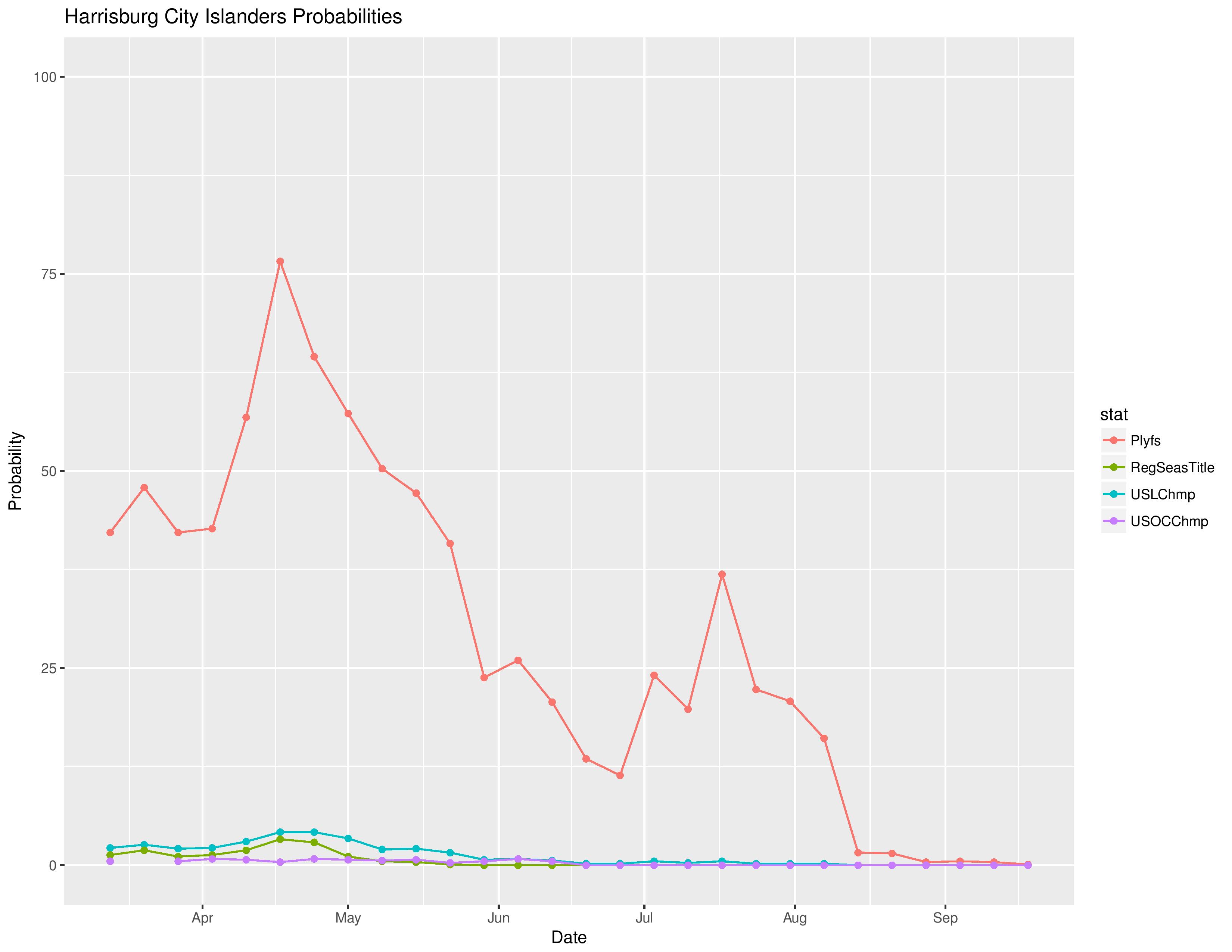
Bethlehem’s odds at becoming the USL Champion decreased from 1.0% to 0.9% while Harrisburg City’s chances remains at practically zero:
Over time, we can see how the odds for different prizes change for Bethlehem and Harrisburg.

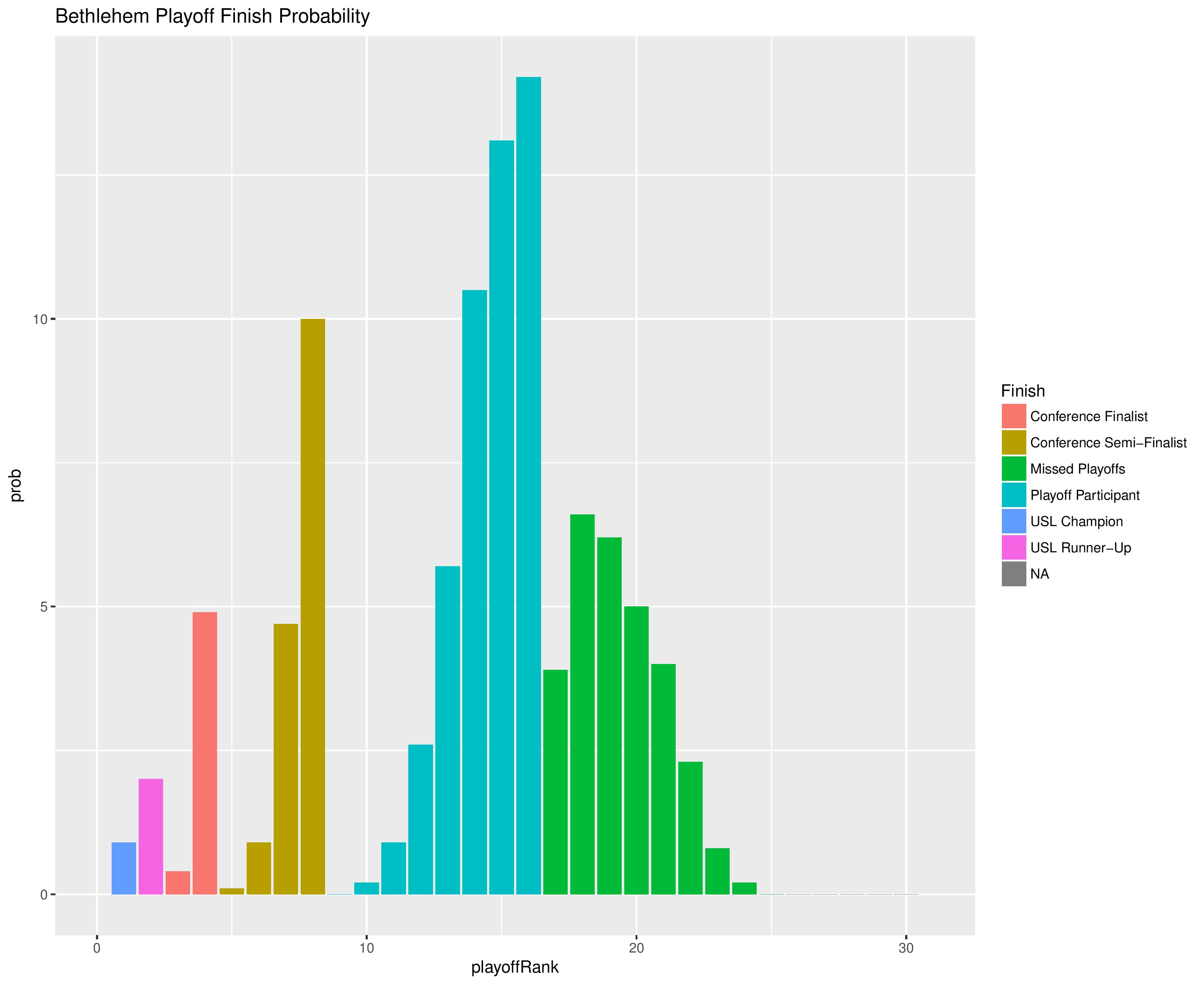
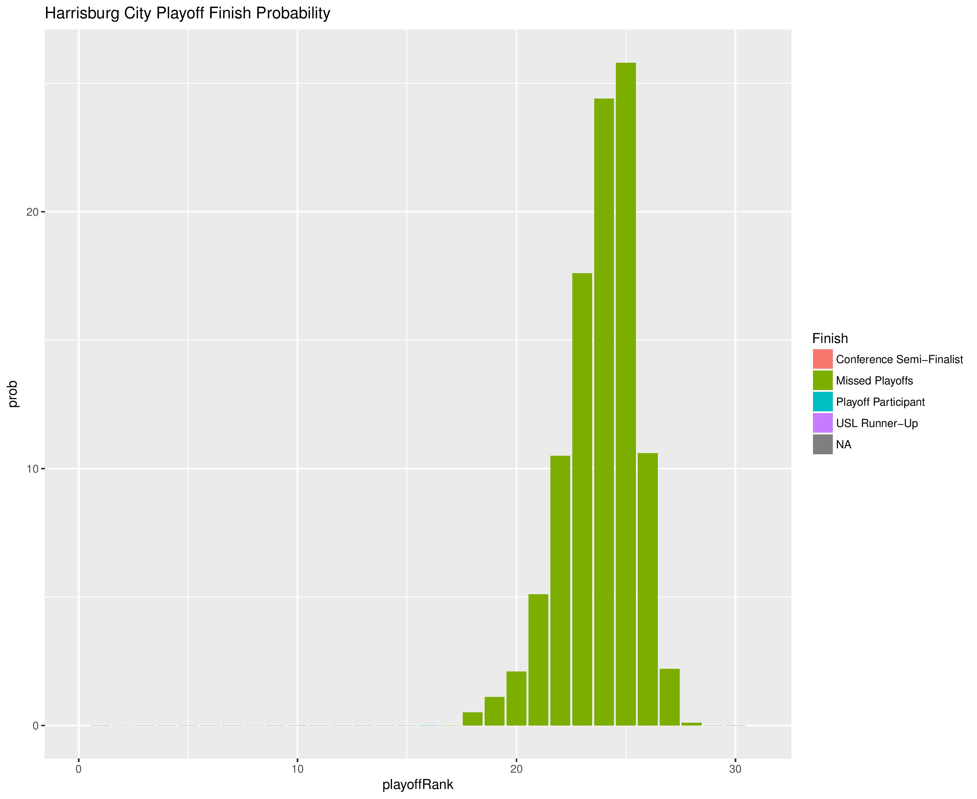
The following shows the probability of each post-playoff ranking finish:
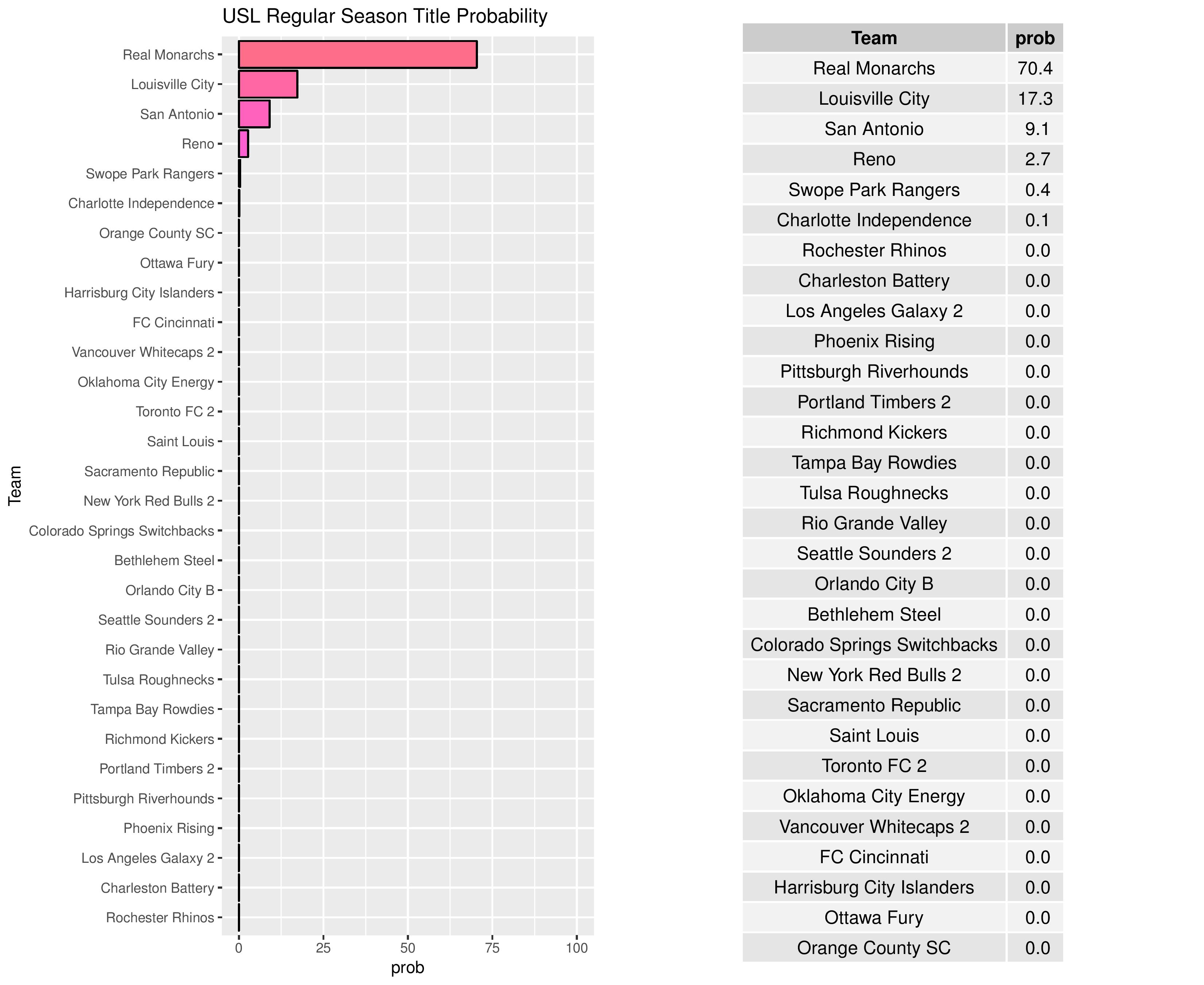
The following shows the summary of simulations in an easy table format.


We can also show how the Remaining Strength of Schedule affects each team.
The “Points Percentage Advantage” shown on the X-axis represents the percentage of points expected over the league average schedule. This “points expected” value is generated by simulating how all teams would perform with all remaining schedules (and therefore judges a schedule based upon how all teams would perform in that scenario).
In short, the higher the value, the easier the remaining schedule.
Remaining home field advantage will make a large contribution here. It can also be true that a better team has an ‘easier’ schedule simply because they do not have to play themselves. Likewise, a bad team may have a ‘harder’ schedule because they also do not play themselves.
The table following the chart also shares helpful context with these percentages.
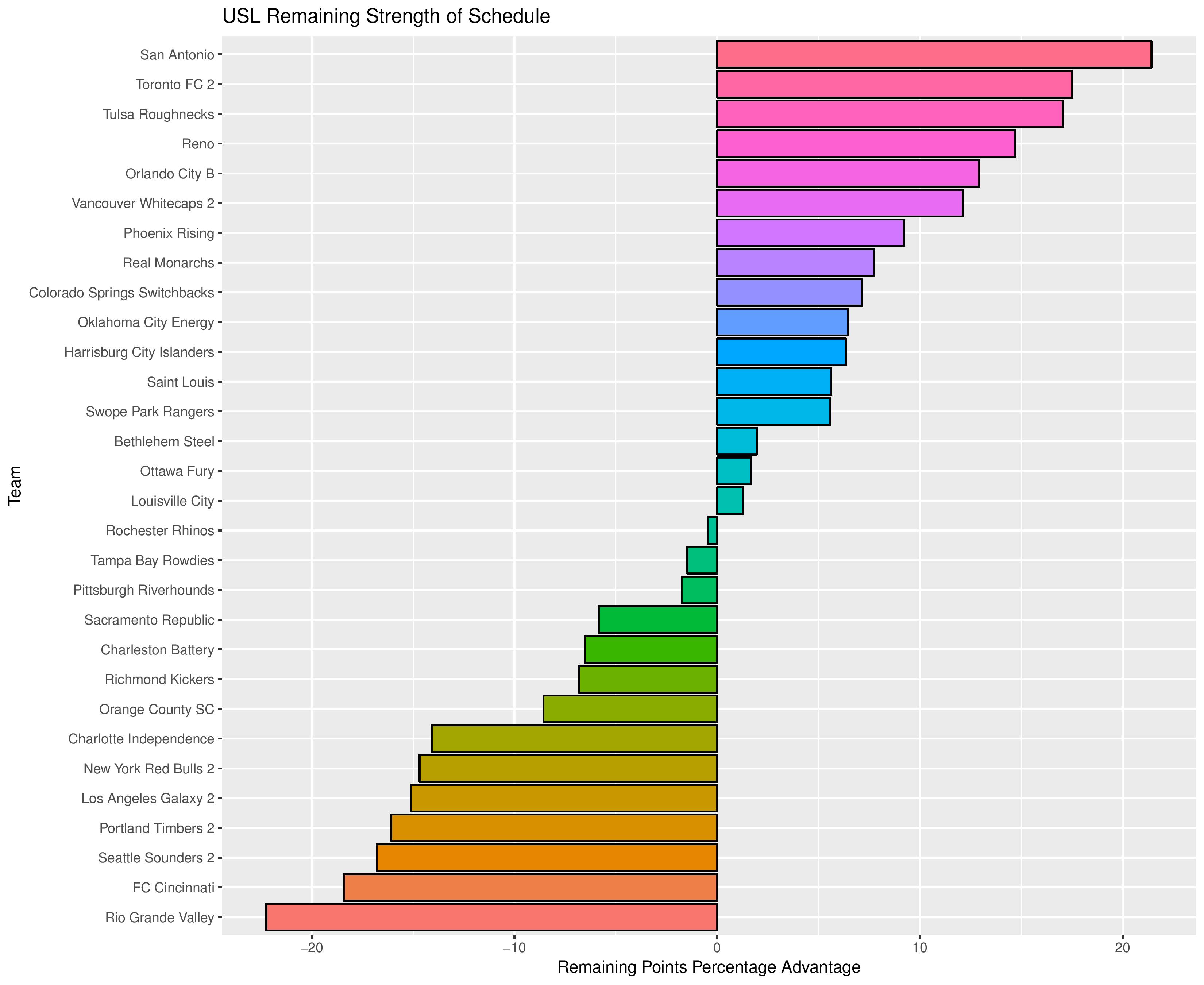
Accompanying the advantage percentage in the following table is their current standings rank (right now ties are not properly calculated beyond pts/gd/gf), the remaining home matches, the remaining away matches, the current average points-per-game of future opponents (results-based, not model-based), and the average power ranking of future opponents according to SEBA.
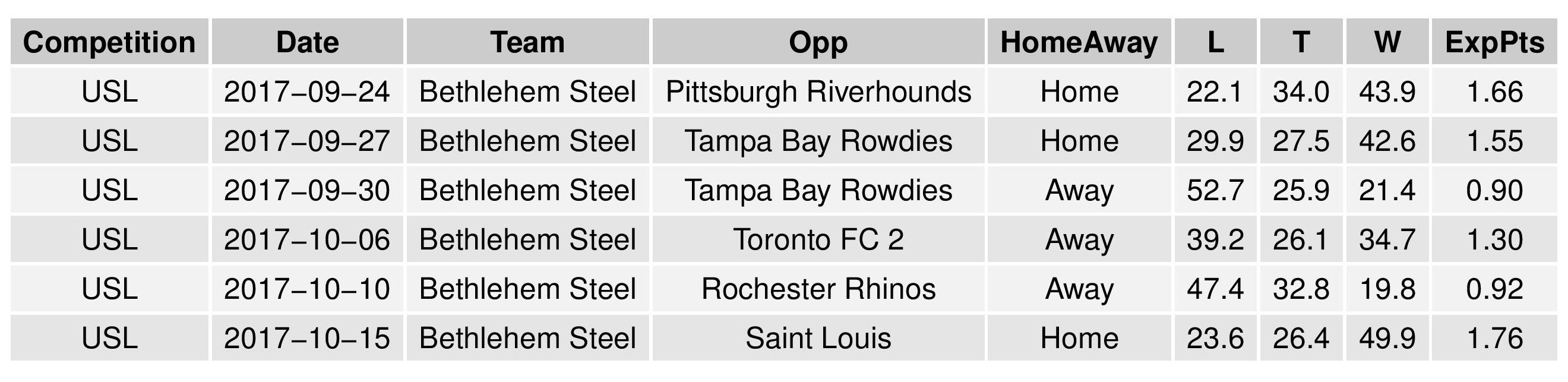
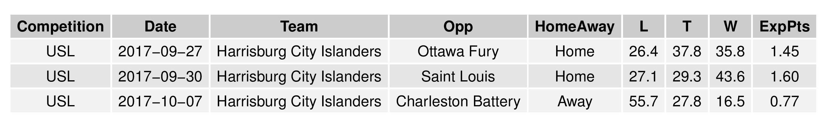
The following shows the expectations for upcoming matches for both Bethlehem and Harrisburg:
Model Validation
This chart is the same as that in the MLS forecast (except for USL matches instead of MLS).
Remember that these data points are not fixed until the end of the season.

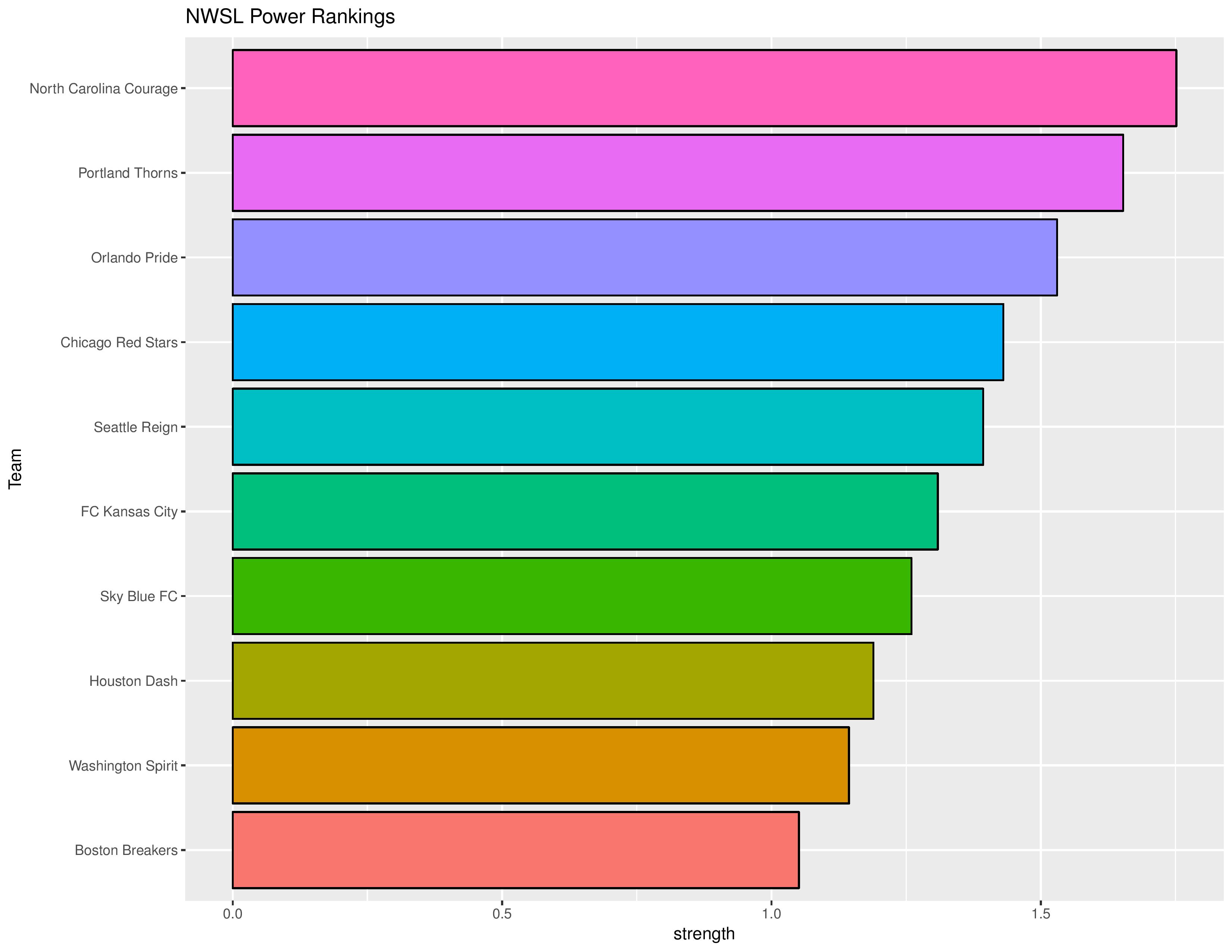
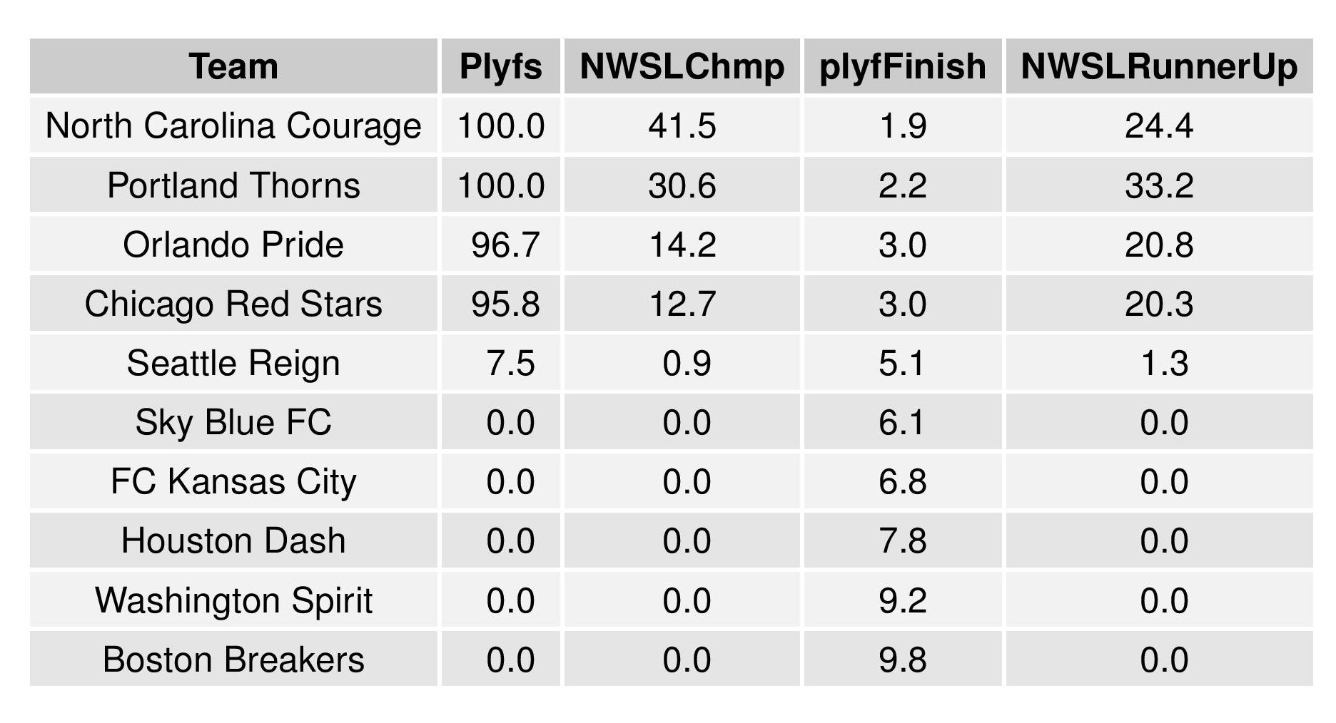
NWSL
Power Rankings
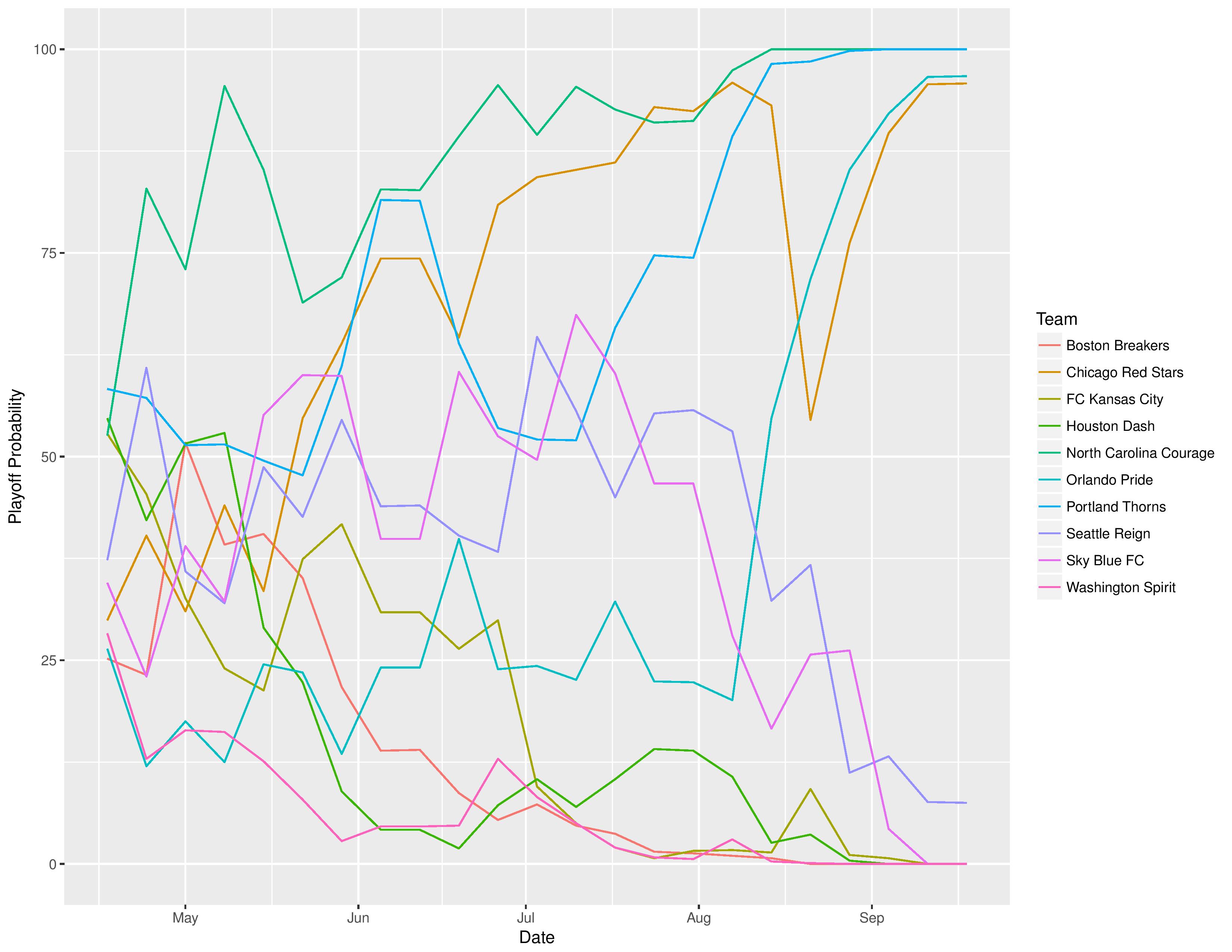
Playoffs probability and more
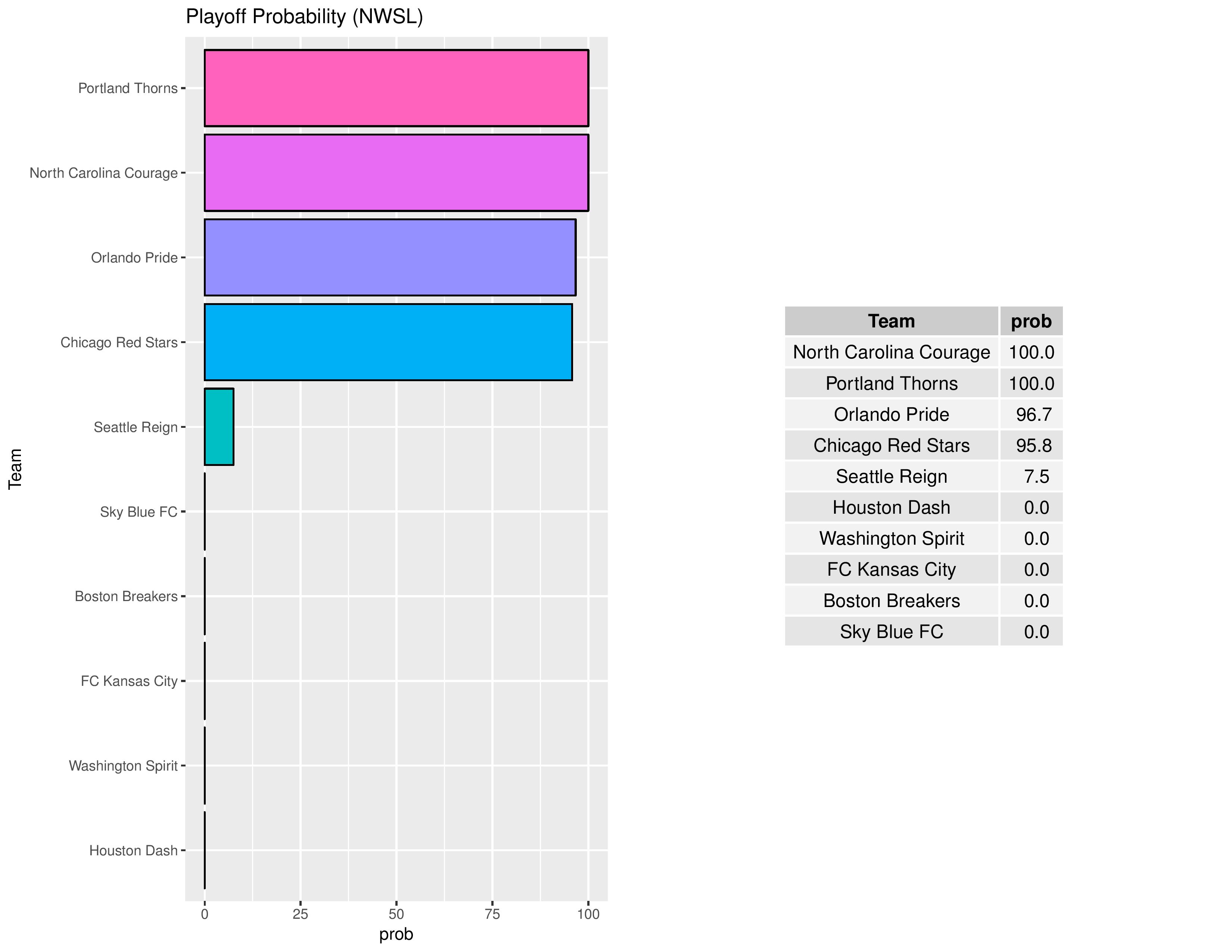
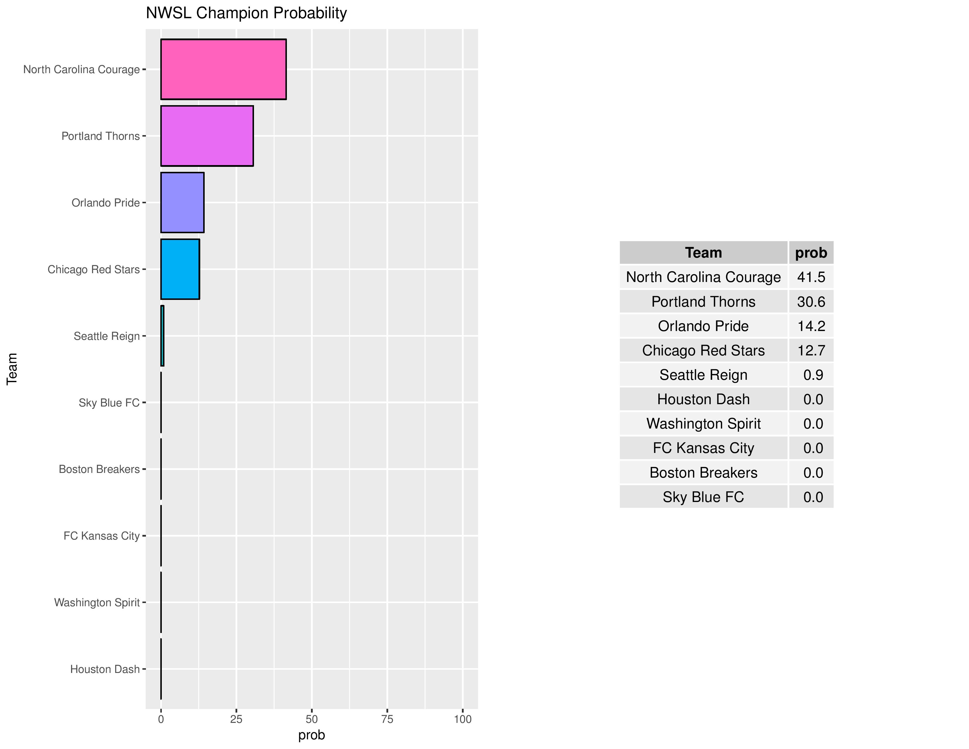

The following shows the summary of the simulations in an easy table format.

As a new feature, we can also show how the Remaining Strength of Schedule affects each team.
The “Points Percentage Advantage” shown on the X-axis represents the percentage of points expected over the league average schedule. This “points expected” value is generated by simulating how all teams would perform with all remaining schedules (and therefore judges a schedule based upon how all teams would perform in that scenario).
In short, the higher the value, the easier the remaining schedule.
It can also be true that a better team has an ‘easier’ schedule simply because they do not have to play themselves. Likewise, a bad team may have a ‘harder’ schedule because they also do not play themselves.
The table following the chart also shares helpful context with these percentages:
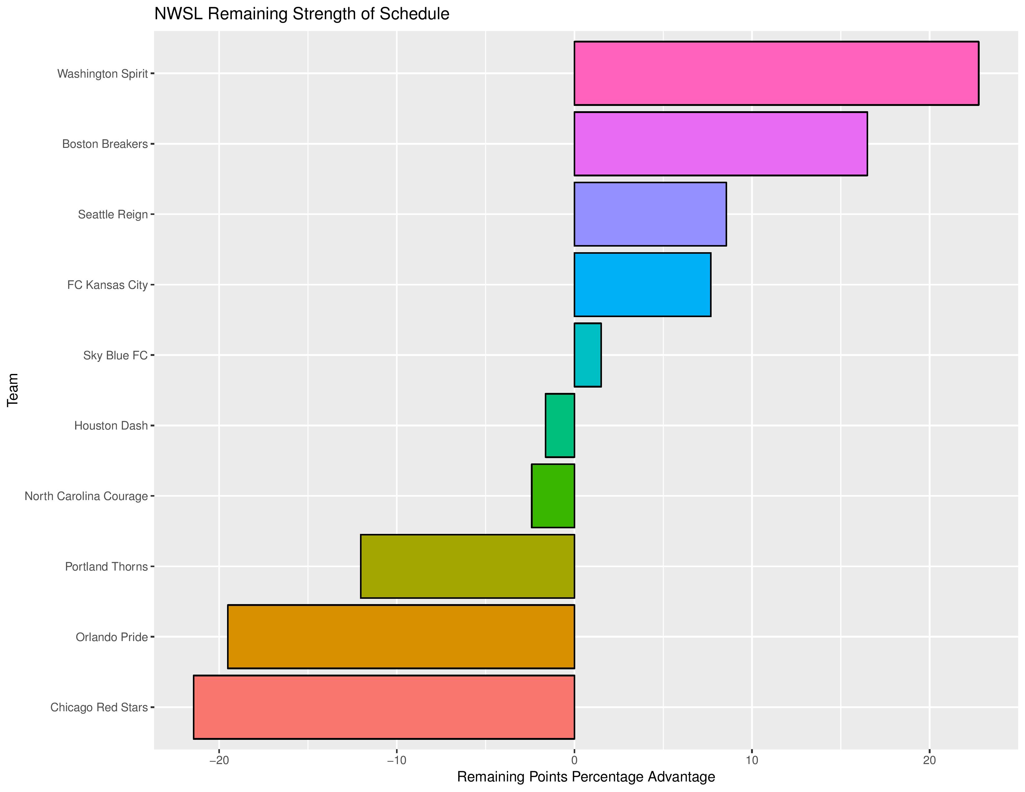
Accompanying the advantage percentage in the following table is their current standings rank (right now ties are not properly calculated beyond pts/gd/gf), the remaining home matches, the remaining away matches, the current average points-per-game of future opponents (results-based, not model-based), and the average power ranking of future opponents according to SEBA.

The SEBA Projection System is an acronym for a tortured collection of words in the Statistical Extrapolation Bayesian Analyzer Projection System. Check out the first season’s post to find out how it works (https://phillysoccerpage.net/2017/03/03/2017-initial-seba-projections/)

I focus most of my attention on the USL and the Steel, I freely admit, when I study these charts and tables.
.
I am less sanguine than the model about Steel results because of the tightness of their closing schedule. They have three in seven days, five days off and then two in five, with the finale coming on the fifth day after that. The three in seven is a real challenge.
.
And my gut rates Pittsburgh Riverhounds a touch more highly than does the computer.